import pandas as pd
import numpy as np
import wooldridge
import statsmodels.formula.api as smf
import matplotlib.pyplot as plt
def report(model, option=3, return_info=False):
summary_table = model.summary2().tables[1]
# Select columns based on the option
if option == 1:
summary = summary_table[["Coef.", "Std.Err."]]
elif option == 2:
summary = summary_table[["Coef.", "Std.Err.", "t"]]
elif option == 3:
summary = summary_table[["Coef.", "Std.Err.", "t", "P>|t|"]]
elif option == 4:
summary = summary_table[["Coef.", "P>|t|"]]
else:
summary = summary_table.copy() # All columns
# Round the values for clean display
summary = summary.round(3)
# Model info
n = int(model.nobs)
r2 = round(model.rsquared, 3)
mse = round(np.sqrt(model.mse_resid), 3)
model_info = f"R² = {r2}, n = {n}, SE = {mse}"
if return_info:
return summary, model_info
else:
print("Model info:", model_info)
return summarywooldridge.data() J.M. Wooldridge (2019) Introductory Econometrics: A Modern Approach,
Cengage Learning, 6th edition.
401k 401ksubs admnrev affairs airfare
alcohol apple approval athlet1 athlet2
attend audit barium beauty benefits
beveridge big9salary bwght bwght2 campus
card catholic cement census2000 ceosal1
ceosal2 charity consump corn countymurders
cps78_85 cps91 crime1 crime2 crime3
crime4 discrim driving earns econmath
elem94_95 engin expendshares ezanders ezunem
fair fertil1 fertil2 fertil3 fish
fringe gpa1 gpa2 gpa3 happiness
hprice1 hprice2 hprice3 hseinv htv
infmrt injury intdef intqrt inven
jtrain jtrain2 jtrain3 kielmc lawsch85
loanapp lowbrth mathpnl meap00_01 meap01
meap93 meapsingle minwage mlb1 mroz
murder nbasal nyse okun openness
pension phillips pntsprd prison prminwge
rdchem rdtelec recid rental return
saving sleep75 slp75_81 smoke traffic1
traffic2 twoyear volat vote1 vote2
voucher wage1 wage2 wagepan wageprc
wine
Examples
wage1 = wooldridge.data("wage1")
gpa1 = wooldridge.data("gpa1")
jtrain = wooldridge.data("jtrain")
hprice1 = wooldridge.data("hprice1")
beauty = wooldridge.data("beauty")
lawsch85 = wooldridge.data("lawsch85")
mlb1 = wooldridge.data("mlb1")
crime1 = wooldridge.data("crime1")
7.1 Hourly Wage Equation
wooldridge.data("wage1", description=True)name of dataset: wage1
no of variables: 24
no of observations: 526
+----------+---------------------------------+
| variable | label |
+----------+---------------------------------+
| wage | average hourly earnings |
| educ | years of education |
| exper | years potential experience |
| tenure | years with current employer |
| nonwhite | =1 if nonwhite |
| female | =1 if female |
| married | =1 if married |
| numdep | number of dependents |
| smsa | =1 if live in SMSA |
| northcen | =1 if live in north central U.S |
| south | =1 if live in southern region |
| west | =1 if live in western region |
| construc | =1 if work in construc. indus. |
| ndurman | =1 if in nondur. manuf. indus. |
| trcommpu | =1 if in trans, commun, pub ut |
| trade | =1 if in wholesale or retail |
| services | =1 if in services indus. |
| profserv | =1 if in prof. serv. indus. |
| profocc | =1 if in profess. occupation |
| clerocc | =1 if in clerical occupation |
| servocc | =1 if in service occupation |
| lwage | log(wage) |
| expersq | exper^2 |
| tenursq | tenure^2 |
+----------+---------------------------------+
These are data from the 1976 Current Population Survey, collected by
Henry Farber when he and I were colleagues at MIT in 1988.
model01 = smf.ols("wage ~ female + educ + exper + tenure", data=wage1).fit()
report(model01)Men [Female = 0 ] has a negative intercept of -1.57 which isn’t useful as no one has control variables with values of zero
On average, females with same education, experience and tenure as men earn less than men by $1.81 per hour
model012 = smf.ols("wage ~ female", data=wage1).fit()
report(model012)In this simple model, men earn 2.51 less than men, they earn 4.59$ per hour
The difference between the two groups is statistically significant
Note: simple regression provides an easy way to do comparison of means test but assumes homoscedasticity
7.2 Effects of Computer Ownership on College GPA
wooldridge.data("gpa1", description=True)name of dataset: gpa1
no of variables: 29
no of observations: 141
+----------+--------------------------------+
| variable | label |
+----------+--------------------------------+
| age | in years |
| soph | =1 if sophomore |
| junior | =1 if junior |
| senior | =1 if senior |
| senior5 | =1 if fifth year senior |
| male | =1 if male |
| campus | =1 if live on campus |
| business | =1 if business major |
| engineer | =1 if engineering major |
| colGPA | MSU GPA |
| hsGPA | high school GPA |
| ACT | 'achievement' score |
| job19 | =1 if job <= 19 hours |
| job20 | =1 if job >= 20 hours |
| drive | =1 if drive to campus |
| bike | =1 if bicycle to campus |
| walk | =1 if walk to campus |
| voluntr | =1 if do volunteer work |
| PC | =1 of pers computer at sch |
| greek | =1 if fraternity or sorority |
| car | =1 if own car |
| siblings | =1 if have siblings |
| bgfriend | =1 if boy- or girlfriend |
| clubs | =1 if belong to MSU club |
| skipped | avg lectures missed per week |
| alcohol | avg # days per week drink alc. |
| gradMI | =1 if Michigan high school |
| fathcoll | =1 if father college grad |
| mothcoll | =1 if mother college grad |
+----------+--------------------------------+
Christopher Lemmon, a former MSU undergraduate, collected these data
from a survey he took of MSU students in Fall 1994.
model02 = smf.ols(formula="colGPA ~ PC + hsGPA + ACT", data=gpa1).fit()
report(model02)A student who has pc is expected to score on average 0.16 higher than other students with same ACT and high school GPA scores
hsGPA is statically significant, so dropping it can change the coefficient of PC
7.3 Effects of Training Grants on Hours of Training
wooldridge.data("jtrain", description=True)name of dataset: jtrain
no of variables: 30
no of observations: 471
+----------+---------------------------------+
| variable | label |
+----------+---------------------------------+
| year | 1987, 1988, or 1989 |
| fcode | firm code number |
| employ | # employees at plant |
| sales | annual sales, $ |
| avgsal | average employee salary |
| scrap | scrap rate (per 100 items) |
| rework | rework rate (per 100 items) |
| tothrs | total hours training |
| union | =1 if unionized |
| grant | = 1 if received grant |
| d89 | = 1 if year = 1989 |
| d88 | = 1 if year = 1988 |
| totrain | total employees trained |
| hrsemp | tothrs/totrain |
| lscrap | log(scrap) |
| lemploy | log(employ) |
| lsales | log(sales) |
| lrework | log(rework) |
| lhrsemp | log(1 + hrsemp) |
| lscrap_1 | lagged lscrap; missing 1987 |
| grant_1 | lagged grant; assumed 0 in 1987 |
| clscrap | lscrap - lscrap_1; year > 1987 |
| cgrant | grant - grant_1 |
| clemploy | lemploy - lemploy[_n-1] |
| clsales | lavgsal - lavgsal[_n-1] |
| lavgsal | log(avgsal) |
| clavgsal | lavgsal - lavgsal[_n-1] |
| cgrant_1 | cgrant[_n-1] |
| chrsemp | hrsemp - hrsemp[_n-1] |
| clhrsemp | lhrsemp - lhrsemp[_n-1] |
+----------+---------------------------------+
H. Holzer, R. Block, M. Cheatham, and J. Knott (1993), “Are Training
Subsidies Effective? The Michigan Experience,” Industrial and Labor
Relations Review 46, 625-636. The authors kindly provided the data.
df = jtrain.copy()
df = df[df["year"] == 1988]
model03 = smf.ols("hrsemp ~ grant + lsales + lemploy", data=df).fit()
report(model03)We used hrsemp in level form because it is zero in many rows
grant is statistically significant with a large coefficient
7.4 Housing Price Regression
wooldridge.data("hprice1", description=True)name of dataset: hprice1
no of variables: 10
no of observations: 88
+----------+------------------------------+
| variable | label |
+----------+------------------------------+
| price | house price, $1000s |
| assess | assessed value, $1000s |
| bdrms | number of bdrms |
| lotsize | size of lot in square feet |
| sqrft | size of house in square feet |
| colonial | =1 if home is colonial style |
| lprice | log(price) |
| lassess | log(assess |
| llotsize | log(lotsize) |
| lsqrft | log(sqrft) |
+----------+------------------------------+
Collected from the real estate pages of the Boston Globe during 1990.
These are homes that sold in the Boston, MA area.
model04 = smf.ols("lprice ~ llotsize + lsqrft + bdrms + colonial", data=hprice1).fit()
report(model04)Controlling for lotsize, bdrms, sqrft, colonial style house is priced more than non colonial style house
7.5 Log Hourly Wage Equation
model05 = smf.ols(
    "lwage ~ female + educ + exper + expersq + tenure + tenursq", data=wage1
).fit()
report(model05)Controlling for educ, exper, tenure, women earn less than men by around 29.7%
A better approximation is
, women earn less than comparable men by 25.7%
7.6 Log Hourly Wage Equation
wooldridge.data("wage1", description=True)name of dataset: wage1
no of variables: 24
no of observations: 526
+----------+---------------------------------+
| variable | label |
+----------+---------------------------------+
| wage | average hourly earnings |
| educ | years of education |
| exper | years potential experience |
| tenure | years with current employer |
| nonwhite | =1 if nonwhite |
| female | =1 if female |
| married | =1 if married |
| numdep | number of dependents |
| smsa | =1 if live in SMSA |
| northcen | =1 if live in north central U.S |
| south | =1 if live in southern region |
| west | =1 if live in western region |
| construc | =1 if work in construc. indus. |
| ndurman | =1 if in nondur. manuf. indus. |
| trcommpu | =1 if in trans, commun, pub ut |
| trade | =1 if in wholesale or retail |
| services | =1 if in services indus. |
| profserv | =1 if in prof. serv. indus. |
| profocc | =1 if in profess. occupation |
| clerocc | =1 if in clerical occupation |
| servocc | =1 if in service occupation |
| lwage | log(wage) |
| expersq | exper^2 |
| tenursq | tenure^2 |
+----------+---------------------------------+
These are data from the 1976 Current Population Survey, collected by
Henry Farber when he and I were colleagues at MIT in 1988.
df = wage1.copy()
df["marrmale"] = ((df["female"] == 0) & (df["married"] == 1)).astype(int)
df["marrfem"] = ((df["female"] == 1) & (df["married"] == 1)).astype(int)
df["singfem"] = ((df["female"] == 1) & (df["married"] == 0)).astype(int)
model06 = smf.ols(
"lwage ~ marrmale + marrfem + singfem + educ + exper + expersq + tenure + tenursq",
data=df,
).fit()
report(model06)All the coefficients are statistically significant. Base group for the dummy variables is single males.
Married men are expected to earn more than single men by 21.3% with the same education, experience and tenure, while married women earns 19.8% less
7.7 Effects of Physical Attractiveness on Wage
wooldridge.data("beauty", description=True)name of dataset: beauty
no of variables: 17
no of observations: 1260
+----------+-------------------------------+
| variable | label |
+----------+-------------------------------+
| wage | hourly wage |
| lwage | log(wage) |
| belavg | =1 if looks <= 2 |
| abvavg | =1 if looks >=4 |
| exper | years of workforce experience |
| looks | from 1 to 5 |
| union | =1 if union member |
| goodhlth | =1 if good health |
| black | =1 if black |
| female | =1 if female |
| married | =1 if married |
| south | =1 if live in south |
| bigcity | =1 if live in big city |
| smllcity | =1 if live in small city |
| service | =1 if service industry |
| expersq | exper^2 |
| educ | years of schooling |
+----------+-------------------------------+
Hamermesh, D.S. and J.E. Biddle (1994), “Beauty and the Labor Market,”
American Economic Review 84, 1174-1194. Professor Hamermesh kindly
provided me with the data. For manageability, I have included only a
subset of the variables, which results in somewhat larger sample sizes
than reported for the regressions in the Hamermesh and Biddle paper.
7.8 Effects of Law School Rankings on Starting Salaries
wooldridge.data("lawsch85", description=True)name of dataset: lawsch85
no of variables: 21
no of observations: 156
+----------+----------------------------+
| variable | label |
+----------+----------------------------+
| rank | law school ranking |
| salary | median starting salary |
| cost | law school cost |
| LSAT | median LSAT score |
| GPA | median college GPA |
| libvol | no. volumes in lib., 1000s |
| faculty | no. of faculty |
| age | age of law sch., years |
| clsize | size of entering class |
| north | =1 if law sch in north |
| south | =1 if law sch in south |
| east | =1 if law sch in east |
| west | =1 if law sch in west |
| lsalary | log(salary) |
| studfac | student-faculty ratio |
| top10 | =1 if ranked in top 10 |
| r11_25 | =1 if ranked 11-25 |
| r26_40 | =1 if ranked 26-40 |
| r41_60 | =1 if ranked 41-60 |
| llibvol | log(libvol) |
| lcost | log(cost) |
+----------+----------------------------+
Collected by Kelly Barnett, an MSU economics student, for use in a
term project. The data come from two sources: The Official Guide to
U.S. Law Schools, 1986, Law School Admission Services, and The Gourman
Report: A Ranking of Graduate and Professional Programs in American
and International Universities, 1995, Washington, D.C.
df = lawsch85.copy()
df["top10"] = (df["rank"] <= 10).astype(int)
df["r11_25"] = ((df["rank"] > 10) & (df["rank"] <= 25)).astype(int)
df["r26_40"] = ((df["rank"] > 25) & (df["rank"] <= 40)).astype(int)
df["r41_60"] = ((df["rank"] > 40) & (df["rank"] <= 60)).astype(int)
df["r61_100"] = ((df["rank"] > 60) & (df["rank"] <= 100)).astype(int)
bins = [0, 10, 25, 40, 60, 100, lawsch85["rank"].max()]
labels = ["Top 10", "11–25", "26–40", "41–60", "61–100", "101+"]
lawsch85["rank_group"] = pd.cut(lawsch85["rank"], bins=bins, labels=labels, right=True)
rank_group_counts = lawsch85["rank_group"].value_counts().sort_index()
rank_group_counts.plot(kind="bar", color="navy", edgecolor="black")
plt.xlabel("School Rank Group")
plt.ylabel("Number of Schools")
plt.title("Number of Law Schools by Rank Group")
plt.xticks(rotation=45)
plt.tight_layout()
plt.show()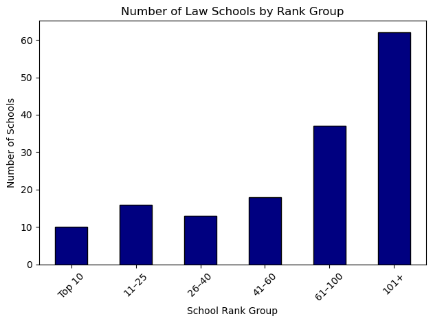
model08 = smf.ols(
    "lsalary ~ top10 + r11_25 + r26_40 + r41_60 + r61_100 + LSAT + GPA + llibvol + lcost",
    data=df,
).fit()
report(model08)Schools below 100 is left as the base group.
All the ranks are statistically significant controlling for .
The difference between is relatively small, so using the approximation: Schools ranked 61 to 100 earn a median salary 13.2% higher than schools ranked 101+
Using exact formula with top10: : Top 10 schools earn a median salary 100% higher than schools below 100.
Note: Rank of a school depends on other schools, so random sample assumption is violated. As long as the error term is uncorrelated with the explanatory variables, there is no problem caused.
7.9 Effects of Computer Usage on Wages
I will simulate the data because its not available
np.random.seed(42)

# Sample size
n = 13379

# Binary indicators
compwork = np.random.binomial(1, 0.3, n)
comphome = np.random.binomial(1, 0.2, n)
interaction = compwork * comphome

# Target betas
beta0 = 1
beta1 = 0.177
beta2 = 0.070
beta3 = 0.017

# To hit target SEs approximately, set noise level accordingly
# After experimentation, this works well
sigma = 0.05  # Adjust noise scale

# Generate lwage
error = np.random.normal(0, sigma, n)
lwage = beta0 + beta1 * compwork + beta2 * comphome + beta3 * interaction + error

# Create DataFrame
df = pd.DataFrame({"lwage": lwage, "compwork": compwork, "comphome": comphome})

# Interaction term
df["interaction"] = df["compwork"] * df["comphome"]
model09 = smf.ols("lwage ~ compwork + comphome + interaction", data=df).fit()
report(model09)Base group is people who don’t use computer at home nor work.
Using computer at work only results in more wage than base group by 17.7%.
Using computer at home only results in more wage than base group by 7.1%.
Using computer at both places results in more wage than base group by
or more accurately 30.2%
(0.177 + 0.071 + 0.016) * 100, np.exp(0.177 + 0.071 + 0.016) - 1(26.400000000000002, np.float64(0.30212819630089416))7.10 Log Hourly Wage Equation
female*educ results in female, educ, interaction
female:educ results in interaction
model010 = smf.ols(
    "lwage ~ female*educ  + exper + expersq + tenure + tenursq ", data=wage1
).fit()
report(model010)# Generate prediction data
educ_range = np.linspace(wage1["educ"].min(), wage1["educ"].max(), 100)
# Create a DataFrame with two groups: male (female=0) and female (female=1)
pred_data = pd.DataFrame(
{
"educ": np.tile(educ_range, 2),
"female": np.repeat([0, 1], len(educ_range)),
}
)
# Add mean values for other covariates
for var in ["exper", "expersq", "tenure", "tenursq"]:
pred_data[var] = wage1[var].mean()
# Compute interaction term
pred_data["female:educ"] = pred_data["female"] * pred_data["educ"]
# Predict log wages
pred_data["lwage_pred"] = model010.predict(pred_data)
# Plot
plt.figure(figsize=(8, 6))
for gender, label in zip([0, 1], ["Male", "Female"]):
subset = pred_data[pred_data["female"] == gender]
plt.plot(subset["educ"], subset["lwage_pred"], label=label)
plt.xlabel("Education (Years)")
plt.ylabel("Predicted log(Wage)")
plt.title("Predicted log(Wage) by Education and Gender")
plt.legend()
plt.grid(True)
plt.show()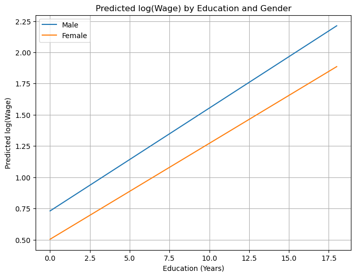
Return on education for men is 8.2%
Return on education for women is
The difference on education between men and women is not statistically significant
female is no longer statistically significant, due to the multicollineairty [strong correlation between female and interaction term, standard error increased]
female coefficient measures salary difference between men and women controlling for education = 0 which is not common. A more useful value for education is the mean in the sample 12.5 [recall chapter 6]
7.11 Effects of Race on Baseball Player Salaries
wooldridge.data("mlb1", description=True)name of dataset: mlb1
no of variables: 47
no of observations: 353
+----------+----------------------------+
| variable | label |
+----------+----------------------------+
| salary | 1993 season salary |
| teamsal | team payroll |
| nl | =1 if national league |
| years | years in major leagues |
| games | career games played |
| atbats | career at bats |
| runs | career runs scored |
| hits | career hits |
| doubles | career doubles |
| triples | career triples |
| hruns | career home runs |
| rbis | career runs batted in |
| bavg | career batting average |
| bb | career walks |
| so | career strike outs |
| sbases | career stolen bases |
| fldperc | career fielding perc |
| frstbase | = 1 if first base |
| scndbase | =1 if second base |
| shrtstop | =1 if shortstop |
| thrdbase | =1 if third base |
| outfield | =1 if outfield |
| catcher | =1 if catcher |
| yrsallst | years as all-star |
| hispan | =1 if hispanic |
| black | =1 if black |
| whitepop | white pop. in city |
| blackpop | black pop. in city |
| hisppop | hispanic pop. in city |
| pcinc | city per capita income |
| gamesyr | games per year in league |
| hrunsyr | home runs per year |
| atbatsyr | at bats per year |
| allstar | perc. of years an all-star |
| slugavg | career slugging average |
| rbisyr | rbis per year |
| sbasesyr | stolen bases per year |
| runsyr | runs scored per year |
| percwhte | percent white in city |
| percblck | percent black in city |
| perchisp | percent hispanic in city |
| blckpb | black*percblck |
| hispph | hispan*perchisp |
| whtepw | white*percwhte |
| blckph | black*perchisp |
| hisppb | hispan*percblck |
| lsalary | log(salary) |
+----------+----------------------------+
Collected by G. Mark Holmes, a former MSU undergraduate, for a term
project. The salary data were obtained from the New York Times, April
11, 1993. The baseball statistics are from The Baseball Encyclopedia,
9th edition, and the city population figures are from the Statistical
Abstract of the United States.
df = mlb1.copy()
df = df[(df["percblck"] != 0)]
model011 = smf.ols(
"lsalary ~ years + gamesyr + bavg + hrunsyr + rbisyr + runsyr + fldperc + allstar + black + hispan + black:percblck + hispan:perchisp",
data=df,
).fit()
report(model011)The base group is white players
model011.f_test("black=0, hispan=0, black:percblck=0, hispan:perchisp=0")<class 'statsmodels.stats.contrast.ContrastResults'>
<F test: F=2.647888304563977, p=0.03347614735675824, df_denom=317, df_num=4>The race variables are statistically significant
black coefficient: if a black player plays in a city with no blacks [perclck = 0], he earns 19.8% less than white players.
black:percblck: if percentage of black increase by 10%, holding percentage of hispanic fixed [white percentage decreases by 10% as base group], wage increases by 1.2% and the black player earns [-0.198 + (0.0125*10)*100 =] 7.3% less than white players
To find percentage of hispanic that makes hispanic players earn as white people, solve for [-0.190 + 0.0201 perchisp = 0] to get perchisp = 9.45
Note: these findings can’t prove discrimination, good black players prefer staying in cities with big black percentage.
7.12 A Linear Probability Model of Arrests
wooldridge.data("crime1", description=True)name of dataset: crime1
no of variables: 16
no of observations: 2725
+----------+---------------------------------+
| variable | label |
+----------+---------------------------------+
| narr86 | # times arrested, 1986 |
| nfarr86 | # felony arrests, 1986 |
| nparr86 | # property crme arr., 1986 |
| pcnv | proportion of prior convictions |
| avgsen | avg sentence length, mos. |
| tottime | time in prison since 18 (mos.) |
| ptime86 | mos. in prison during 1986 |
| qemp86 | # quarters employed, 1986 |
| inc86 | legal income, 1986, $100s |
| durat | recent unemp duration |
| black | =1 if black |
| hispan | =1 if Hispanic |
| born60 | =1 if born in 1960 |
| pcnvsq | pcnv^2 |
| pt86sq | ptime86^2 |
| inc86sq | inc86^2 |
+----------+---------------------------------+
J. Grogger (1991), “Certainty vs. Severity of Punishment,” Economic
Inquiry 29, 297-309. Professor Grogger kindly provided a subset of the
data he used in his article.
df = crime1.copy()
df["arr86"] = (df["narr86"] > 0).astype(int)
model012 = smf.ols("arr86 ~ pcnv + avgsen + tottime + ptime86 + qemp86", data=df).fit()
report(model012)model012.f_test("avgsen = 0, tottime=0")<class 'statsmodels.stats.contrast.ContrastResults'>
<F test: F=1.059700444036282, p=0.346702695391494, df_denom=2.72e+03, df_num=2>intercept: probability of someone being arrested with no convictions is 0.441
avgsen, tottime: insignificant individually and jointly
ptime86: if a man is in prison for 12 months, probability of arrest is [0.441 - 0.22*12] = 0.177, which should be zero cuz he can’t be arrested while already in prison
qemp86: if a man is employed for 12 months, he is [-0.043*4 = 0.172] less likely to be arrested than a man who is no employed