import wooldridge
import pandas as pd
wooldridge.data() J.M. Wooldridge (2019) Introductory Econometrics: A Modern Approach,
Cengage Learning, 6th edition.
401k 401ksubs admnrev affairs airfare
alcohol apple approval athlet1 athlet2
attend audit barium beauty benefits
beveridge big9salary bwght bwght2 campus
card catholic cement census2000 ceosal1
ceosal2 charity consump corn countymurders
cps78_85 cps91 crime1 crime2 crime3
crime4 discrim driving earns econmath
elem94_95 engin expendshares ezanders ezunem
fair fertil1 fertil2 fertil3 fish
fringe gpa1 gpa2 gpa3 happiness
hprice1 hprice2 hprice3 hseinv htv
infmrt injury intdef intqrt inven
jtrain jtrain2 jtrain3 kielmc lawsch85
loanapp lowbrth mathpnl meap00_01 meap01
meap93 meapsingle minwage mlb1 mroz
murder nbasal nyse okun openness
pension phillips pntsprd prison prminwge
rdchem rdtelec recid rental return
saving sleep75 slp75_81 smoke traffic1
traffic2 twoyear volat vote1 vote2
voucher wage1 wage2 wagepan wageprc
wine
Computer problems
C1
Use the data in Wage1 for this exercise
wooldridge.data("wage1", description=True)name of dataset: wage1
no of variables: 24
no of observations: 526
+----------+---------------------------------+
| variable | label |
+----------+---------------------------------+
| wage | average hourly earnings |
| educ | years of education |
| exper | years potential experience |
| tenure | years with current employer |
| nonwhite | =1 if nonwhite |
| female | =1 if female |
| married | =1 if married |
| numdep | number of dependents |
| smsa | =1 if live in SMSA |
| northcen | =1 if live in north central U.S |
| south | =1 if live in southern region |
| west | =1 if live in western region |
| construc | =1 if work in construc. indus. |
| ndurman | =1 if in nondur. manuf. indus. |
| trcommpu | =1 if in trans, commun, pub ut |
| trade | =1 if in wholesale or retail |
| services | =1 if in services indus. |
| profserv | =1 if in prof. serv. indus. |
| profocc | =1 if in profess. occupation |
| clerocc | =1 if in clerical occupation |
| servocc | =1 if in service occupation |
| lwage | log(wage) |
| expersq | exper^2 |
| tenursq | tenure^2 |
+----------+---------------------------------+
These are data from the 1976 Current Population Survey, collected by
Henry Farber when he and I were colleagues at MIT in 1988.
wage = wooldridge.data("wage1")
wage.head()(i) Find the average education level in the sample. What are the lowest and highest years of education?
wage["educ"].describe()count 526.000000
mean 12.562738
std 2.769022
min 0.000000
25% 12.000000
50% 12.000000
75% 14.000000
max 18.000000
Name: educ, dtype: float64Average years of education is 12.56, minimum years of education is 0 and maximum is 18
(ii) Find the average hourly wage in the sample.
wage["wage"].mean()np.float64(5.896102674787035)The wage in 1976 had an average 5.9
(iii) How many women are in the sample? How many men?
wage.columnsIndex(['wage', 'educ', 'exper', 'tenure', 'nonwhite', 'female', 'married',
'numdep', 'smsa', 'northcen', 'south', 'west', 'construc', 'ndurman',
'trcommpu', 'trade', 'services', 'profserv', 'profocc', 'clerocc',
'servocc', 'lwage', 'expersq', 'tenursq'],
dtype='object')wage.female.value_counts()female
0 274
1 252
Name: count, dtype: int64There are 274 males and 252 females in the dataset
C2
Use the data in BWGHT to answer this question.
wooldridge.data("bwght", description=True)name of dataset: bwght
no of variables: 14
no of observations: 1388
+----------+--------------------------------+
| variable | label |
+----------+--------------------------------+
| faminc | 1988 family income, $1000s |
| cigtax | cig. tax in home state, 1988 |
| cigprice | cig. price in home state, 1988 |
| bwght | birth weight, ounces |
| fatheduc | father's yrs of educ |
| motheduc | mother's yrs of educ |
| parity | birth order of child |
| male | =1 if male child |
| white | =1 if white |
| cigs | cigs smked per day while preg |
| lbwght | log of bwght |
| bwghtlbs | birth weight, pounds |
| packs | packs smked per day while preg |
| lfaminc | log(faminc) |
+----------+--------------------------------+
J. Mullahy (1997), “Instrumental-Variable Estimation of Count Data
Models: Applications to Models of Cigarette Smoking Behavior,” Review
of Economics and Statistics 79, 596-593. Professor Mullahy kindly
provided the data. He obtained them from the 1988 National Health
Interview Survey.
df2 = wooldridge.data("bwght")
df2.head()(i) How many women are in the sample, and how many report smoking during pregnancy?
len(df2)1388df2[df2["cigs"] != 0].shape[0]212df2[df2["cigs"] != 0].shape[0] / len(df2)0.15273775216138327There are 1388 women in the dataset, 212 of them reported smoking during pregnancy which repesents of the women in the dataset
(ii) What is the average number of cigarettes smoked per day? Is the average a good measure of the“typical” woman in this case? Explain.
df2["cigs"].value_counts().sort_index().plot(kind="bar")<Axes: xlabel='cigs'>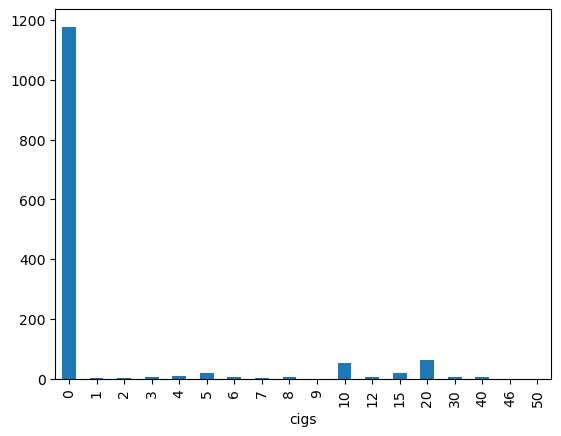
df2[df2["cigs"] != 0]["cigs"].value_counts().sort_index().plot(kind="bar")<Axes: xlabel='cigs'>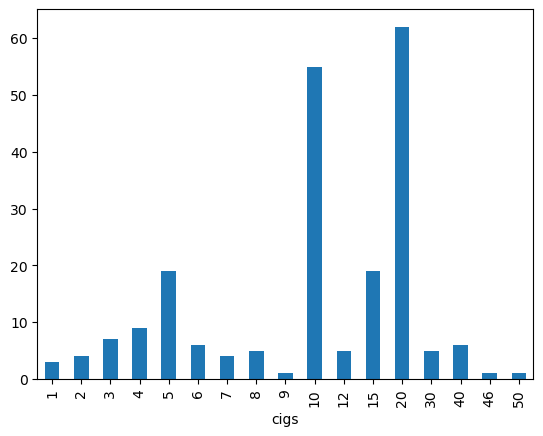
df2["cigs"].mean()np.float64(2.0871757925072045)df2[df2["cigs"] != 0]["cigs"].mean()np.float64(13.665094339622641)Average ciggaretes per day is roughly 2 but its not representative cuz it is zero inflated. 1176 women did not smoke representing of the data. If the zero inflation is removed, average becomes 13.7
(iii) Among women who smoked during pregnancy, what is the average number of cigarettes
The average ciggaretes consumed by women who smoke during pregnancy is 13.7 ciggaretes per day
(iv) Find the average of fatheduc in the sample. Why are only 1,192 observations used to compute this average?
df2["fatheduc"].value_counts().sort_index().plot(kind="bar")<Axes: xlabel='fatheduc'>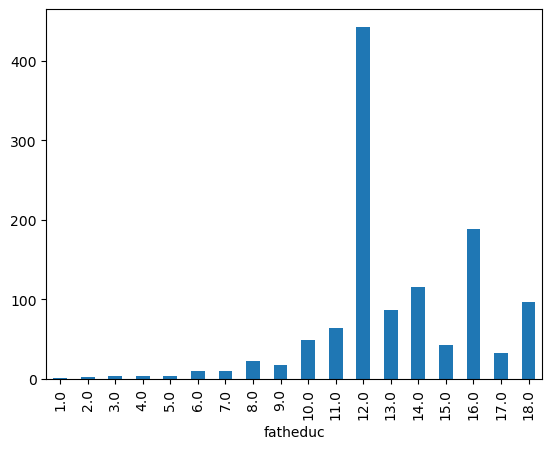
df2["fatheduc"].describe()count 1192.000000
mean 13.186242
std 2.745985
min 1.000000
25% 12.000000
50% 12.000000
75% 16.000000
max 18.000000
Name: fatheduc, dtype: float64df2["fatheduc"].isnull().sum()np.int64(196)The average years of education of the fathers is 13.2. This average is based on 1192 father only cuz we have missing data for 196 fathers
(v) Report the average family income and its standard deviation in dollars.
df2["faminc"].mean(), df2["faminc"].std()(np.float64(29.026657060518733), np.float64(18.73928463224534))Average family income is with a standard deviation of
C3
The data in MEAP01 are for the state of Michigan in the year 2001. Use these data to answer the following questions.
wooldridge.data("meap01", description=True)name of dataset: meap01
no of variables: 11
no of observations: 1823
+----------+-----------------------------------------------+
| variable | label |
+----------+-----------------------------------------------+
| dcode | district code |
| bcode | building code |
| math4 | % students satisfactory, 4th grade math |
| read4 | % students satisfactory, 4th grade reading |
| lunch | % students eligible for free or reduced lunch |
| enroll | school enrollment |
| expend | total spending, $ |
| exppp | expenditures per pupil: expend/enroll |
| lenroll | log(enroll) |
| lexpend | log(expend) |
| lexppp | log(exppp) |
+----------+-----------------------------------------------+
Michigan Department of Education, www.michigan.gov/mde
df3 = wooldridge.data("meap01")(i) Find the largest and smallest values of math4. Does the range make sense? Explain
df3["math4"].describe()count 1823.000000
mean 71.908996
std 19.954092
min 0.000000
25% 61.600000
50% 76.400002
75% 87.000000
max 100.000000
Name: math4, dtype: float64The smallest is 0 while the largest is 100. The range between smallest and largest values is massive.
(ii) How many schools have a perfect pass rate on the math test? What percentage is this of the total sample?
df3["math4"].plot(kind="hist", edgecolor="black", density=True, bins=10)<Axes: ylabel='Frequency'>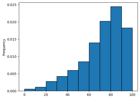
df3[df3["math4"] == 100]["math4"].count()np.int64(38)df3[df3["math4"] == 100]["math4"].count() / len(df3)np.float64(0.020844761382336808)len(df3)182338 out of 1823 schools have a perfect school representing of the dataset
(iii) How many schools have math pass rates of exactly 50%?
df3[df3["math4"] == 50]["math4"].count()np.int64(17)17 schools
(iv) Compare the average pass rates for the math and reading scores. Which test is harder to pass?
df3["math4"].mean(), df3["read4"].mean()(np.float64(71.90899606805154), np.float64(60.06187602862904))Based on average pass rates, reading was harder to pass in 2001
(v) Find the correlation between math4 and read4. What do you conclude?
import numpy as npdf3["math4"].corr(df3["read4"])np.float64(0.8427281457721156)df3.plot(kind="scatter", x="math4", y="read4")<Axes: xlabel='math4', ylabel='read4'>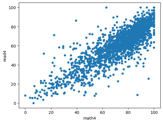
The sample correlation is 0.843 showing high linear association between the two tests. This indicates that schools that have high pass rates on one test is likely to have high pass rates for the other test
(vi) The variable exppp is expenditure per pupil. Find the average of exppp along with its standard deviation. Would you say there is wide variation in per pupil spending?
df3["exppp"].plot(kind="hist", edgecolor="black", density=True)<Axes: ylabel='Frequency'>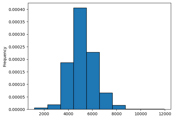
df3["exppp"].mean().round(), df3["exppp"].std().round()(np.float64(5195.0), np.float64(1092.0))The mean is 5195 with a standard variation of 1092 showing high variability in the data
(vii) Suppose School A spends 5,500 per student. By whatpercentage does School A’s spending exceed School B’s? Compare this to 100 · [log(6,000) –log(5,500)]
C4
The data in JTRAIN2 come from a job training experiment conducted for low-income men during 1976–1977; see Lalonde (1986).
wooldridge.data("jtrain2", description=True)name of dataset: jtrain2
no of variables: 19
no of observations: 445
+----------+---------------------------------+
| variable | label |
+----------+---------------------------------+
| train | =1 if assigned to job training |
| age | age in 1977 |
| educ | years of education |
| black | =1 if black |
| hisp | =1 if Hispanic |
| married | =1 if married |
| nodegree | =1 if no high school degree |
| mosinex | # mnths prior to 1/78 in expmnt |
| re74 | real earns., 1974, $1000s |
| re75 | real earns., 1975, $1000s |
| re78 | real earns., 1978, $1000s |
| unem74 | =1 if unem. all of 1974 |
| unem75 | =1 if unem. all of 1975 |
| unem78 | =1 if unem. all of 1978 |
| lre74 | log(re74); zero if re74 == 0 |
| lre75 | log(re75); zero if re75 == 0 |
| lre78 | log(re78); zero if re78 == 0 |
| agesq | age^2 |
| mostrn | months in training |
+----------+---------------------------------+
R.J. Lalonde (1986), “Evaluating the Econometric Evaluations of
Training Programs with Experimental Data,” American Economic Review
76, 604-620. Professor Jeff Biddle, at MSU, kindly passed the data set
along to me. He obtained it from Professor Lalonde.
df4 = wooldridge.data("jtrain2")(i) Use the indicator variable train to determine the fraction of men receiving job training.
df4["train"].value_counts()train
0 260
1 185
Name: count, dtype: int64(df4["train"] == 1).mean()np.float64(0.4157303370786517)185 men recieved the training representing
(ii) The variable re78 is earnings from 1978, measured in thousands of 1982 dollars. Find the averages of re78 for the sample of men receiving job training and the sample not receiving job training. Is the difference economically large?
df4["re78"].groupby(df4["train"]).mean().round(3)train
0 4.555
1 6.349
Name: re78, dtype: float64Men who recieved the training had average earnings of while men who did not recieve the training had an average of
train_0 = df4["re78"].groupby(df4["train"]).mean()[0]
train_1 = df4["re78"].groupby(df4["train"]).mean()[1]

train_0, train_1
(np.float64(4.554802284088845), np.float64(6.349145357189951))(train_1 - train_0) / train_0np.float64(0.39394532653354264)Those who trained has an earnings increase of which is very large
(iii) The variable unem78 is an indicator of whether a man is unemployed or not in 1978. What fraction of the men who received job training are unemployed? What about for men who did not receive job training? Comment on the difference.
df4["unem78"].groupby(df4["train"]).value_counts()train unem78
0 0 168
1 92
1 0 140
1 45
Name: count, dtype: int64df4["unem78"].groupby(df4["train"]).mean().round(3)train
0 0.354
1 0.243
Name: unem78, dtype: float64of those who trained were unemployed, while of those who did noy train were unemployed. The difference in percentages seems large.
From parts (ii) and (iii), does it appear that the job training program was effective? What would make our conclusions more convincing?
The difference in earnings and unemployment is large indicating that training had a positive effect. We need to statistically test the difference to know if its significant or due to random error