2. Functional Forms Of Regression Models

2. Functional Forms Of Regression Models#

suppressPackageStartupMessages({
  library(tidyverse)
  library(tidymodels)
  library(readxl)
  library(multcomp)
  library(car)
})

Cobb Douglas Function#

Log-log model (Double log) (Constant elasticity) (log-linear)#

\begin{align} \text{output} &= \beta_0 \text{labor}^{\beta_1}\text{capital}^{\beta_2}\ \ln \text{output}_i &= \ln \beta_0 + \beta_1 \ln \text{labor}_i + \beta_2 \ln \text{capital}_i +u \end{align}

labor input (worker hours, in thousands),
and capital input (capital expenditure, in thousands of dollars) for the US manufacturing sector.
The data is cross-sectional, covering 50 states and Washington, DC, for the year 2005.

df <- read_excel("data/Table2_1.xls")
head(df)

A tibble: 6 × 12
obs	output	labor	capital	lnoutput	lnlabor	lncapital	lnoutlab	lncaplab	outputstar	capitalstar	laborstar
<dbl>	<dbl>	<dbl>	<dbl>	<dbl>	<dbl>	<dbl>	<dbl>	<dbl>	<dbl>	<dbl>	<dbl>
1	38372840	424471	2689076	17.46286	12.958599	14.80471	4.504261	1.846109	-0.1079874	0.06368887	0.1343891
2	1805427	19895	57997	14.40631	9.898224	10.96815	4.508084	1.069923	-0.9230660	-0.90551400	-0.9410533
3	23736129	206893	2308272	16.98251	12.239957	14.65201	4.742552	2.412053	-0.4342360	-0.07658678	-0.4439759
4	26981983	304055	1376235	17.11068	12.624964	14.13486	4.485716	1.509898	-0.3618868	-0.41991854	-0.1857003
5	217546032	1809756	13554116	19.19792	14.408703	16.42220	4.789218	2.013498	3.8857391	4.06601191	3.8167481
6	19462751	180366	1790751	16.78401	12.102743	14.39815	4.681270	2.295402	-0.5294886	-0.26722449	-0.5144899

model <- lm(lnoutput~ lnlabor+ lncapital, data = df)

tidy(model)
glance(model)

A tibble: 3 × 5
term	estimate	std.error	statistic	p.value
<chr>	<dbl>	<dbl>	<dbl>	<dbl>
(Intercept)	3.8875990	0.39622813	9.811517	4.704731e-13
lnlabor	0.4683318	0.09892588	4.734169	1.980888e-05
lncapital	0.5212795	0.09688703	5.380281	2.183108e-06

A tibble: 1 × 12
r.squared	adj.r.squared	sigma	statistic	p.value	df	logLik	AIC	BIC	deviance	df.residual	nobs
<dbl>	<dbl>	<dbl>	<dbl>	<dbl>	<dbl>	<dbl>	<dbl>	<dbl>	<dbl>	<int>	<int>
0.9641754	0.9626828	0.266752	645.9316	1.996821e-35	2	-3.426703	14.85341	22.58071	3.415518	48	51

interpretation of the coefficient of lnlabor of about 0.47 is that if we increase the labor input by 1%, on average, output goes up by about 0.47 %, holding the capital input constant

interpretation of the coefficient of lncapital of about 0.52 is that if we increase capital input by 1%, on average, the output increases by about 0.52%, holding the labot input constant

tidy_model <- tidy(model)
colnames(tidy_model)
rownames(tidy_model)

'term'
'estimate'
'std.error'
'statistic'
'p.value'

'1'
'2'
'3'

(intercept <- tidy_model[[1,'estimate']])
exp(intercept)

3.88759899084757

48.7935919066084

(beta_1 <- tidy_model[[2, 'estimate']])
(beta_2 <- tidy_model[[3, 'estimate']])

0.468331833346232

0.521279475667115

(return_to_scale <- beta_1 + beta_2)

0.989611309013347

\[ output = 48.79 \text{labour}^{0.47} \text{capital}^{0.51} \]

linear model#

\[ \text{output} = \beta_0 + \beta_1 \text{labor} + \beta_2 \text{capital} \]

model2 <- lm(output~ labor + capital, data = df)
tidy(model2)
glance(model2)

A tibble: 3 × 5
term	estimate	std.error	statistic	p.value
<chr>	<dbl>	<dbl>	<dbl>	<dbl>
(Intercept)	2.336216e+05	1.250364e+06	0.1868428	8.525714e-01
labor	4.798736e+01	7.058245e+00	6.7987660	1.496564e-08
capital	9.951891e+00	9.781165e-01	10.1745459	1.433023e-13

A tibble: 1 × 12
r.squared	adj.r.squared	sigma	statistic	p.value	df	logLik	AIC	BIC	deviance	df.residual	nobs
<dbl>	<dbl>	<dbl>	<dbl>	<dbl>	<dbl>	<dbl>	<dbl>	<dbl>	<dbl>	<int>	<int>
0.9810653	0.9802763	6300694	1243.514	4.510314e-42	2	-869.2846	1746.569	1754.297	1.90554e+15	48	51

tidy_model2 <- tidy(model2)
as.numeric(tidy_model2$estimate)
as.numeric(tidy_model2$p.value)

233621.609858679
47.987358368403
9.95189072306451

0.852571362047071
1.49656436518791e-08
1.43302279569064e-13

If labor input increases by a unit, the average output goes up by about 48 units, holding capital constant

Linear restriction#

\[\beta_1 + \beta_2 = 1\]

\[\beta_1 = 1 - \beta_2 \]

Manual calculation#

\[ \ln \text{output}_i = \ln \beta_0 + \beta_1 \ln \text{labor}_i + \beta_2 \ln \text{capital}_i + u_i \]

\[ \ln \text{output}_i = \ln \beta_0 + (1- \beta_2) \ln \text{labor}_i + \beta_2 \ln \text{capital}_i + u_i\]

\[ \ln \text{output}_i - \ln \text{labor}_i = \ln \beta_0 + \beta_2(\ln \text{capital}_i - \ln \text{labor}_i) + u_i \]

\[\ln \left (\frac{\text{output}_i}{\text{labor}_i} \right) = \ln \beta_0 + \beta_2 \ln \left(\frac{\text{capital}_i}{\text{labor}_i}\right) + u_i \]

\[F = \frac{(\text{RSS}_{R} -\text{RSS}_{UR}) / m}{\text{RSS}_{UR} / (n - k)} \sim F_{m,n-k} \]

$RSS_R$= residual sum of squares from the restricted regression
$RSS_{UR}$= residual sum of squares from the unrestricted regression
$m$ = number of linear restrictions (1 here)
$k$ = number of parameters in the unrestricted regression (3 here)

model3 <- lm(log(output/labor) ~ log(capital/labor), data = df)
tidy(model3)
glance(model3)

A tibble: 2 × 5
term	estimate	std.error	statistic	p.value
<chr>	<dbl>	<dbl>	<dbl>	<dbl>
(Intercept)	3.7562419	0.18536786	20.263717	1.816211e-25
log(capital/labor)	0.5237564	0.09581225	5.466487	1.535206e-06

A tibble: 1 × 12
r.squared	adj.r.squared	sigma	statistic	p.value	df	logLik	AIC	BIC	deviance	df.residual	nobs
<dbl>	<dbl>	<dbl>	<dbl>	<dbl>	<dbl>	<dbl>	<dbl>	<dbl>	<dbl>	<int>	<int>
0.3788227	0.3661456	0.2644047	29.88247	1.535206e-06	1	-3.501733	13.00347	18.79894	3.425582	49	51

summary(model3)

Call:
lm(formula = log(output/labor) ~ log(capital/labor), data = df)

Residuals:
     Min       1Q   Median       3Q      Max 
-0.43644 -0.12465 -0.05083  0.04356  1.23075 

Coefficients:
                   Estimate Std. Error t value Pr(>|t|)    
(Intercept)         3.75624    0.18537  20.264  < 2e-16 ***
log(capital/labor)  0.52376    0.09581   5.466 1.54e-06 ***
---
Signif. codes:  0 '***' 0.001 '**' 0.01 '*' 0.05 '.' 0.1 ' ' 1

Residual standard error: 0.2644 on 49 degrees of freedom
Multiple R-squared:  0.3788,	Adjusted R-squared:  0.3661 
F-statistic: 29.88 on 1 and 49 DF,  p-value: 1.535e-06

anova(model)

A anova: 3 × 5
	Df	Sum Sq	Mean Sq	F value	Pr(>F)
	<int>	<dbl>	<dbl>	<dbl>	<dbl>
lnlabor	1	89.864812	89.86481250	1262.91571	3.933902e-36
lncapital	1	2.059801	2.05980082	28.94742	2.183108e-06
Residuals	48	3.415518	0.07115662	NA	NA

colnames(anova(model))
rownames(anova(model))

'Df'
'Sum Sq'
'Mean Sq'
'F value'
'Pr(>F)'

'lnlabor'
'lncapital'
'Residuals'

(RSSur <- anova(model)["Residuals","Sum Sq"])
(DFur <-anova(model)["Residuals","Df"])

3.41551772437328

48

anova(model3)
(RSSr <- anova(model3)["Residuals","Sum Sq"])

A anova: 2 × 5
	Df	Sum Sq	Mean Sq	F value	Pr(>F)
	<int>	<dbl>	<dbl>	<dbl>	<dbl>
log(capital/labor)	1	2.089079	2.08907903	29.88247	1.535206e-06
Residuals	49	3.425582	0.06990984	NA	NA

3.42558215188511

(f = ((RSSr-RSSur)/1)/(RSSur/(DFur)))

0.141440495864081

(p_value <- pf(f, 1, DFur, lower.tail = FALSE))

0.7085103234663

conclusion: The restirction was correct, can use restricted model

using car package#

unrestricted_model <- lm(log(output) ~ log(labor) + log(capital), data = df)
hypothesis <- "log(labor) + log(capital) = 1"

(test_result <- linearHypothesis(unrestricted_model, hypothesis))

A anova: 2 × 6
	Res.Df	RSS	Df	Sum of Sq	F	Pr(>F)
	<dbl>	<dbl>	<dbl>	<dbl>	<dbl>	<dbl>
1	49	3.425582	NA	NA	NA	NA
2	48	3.415520	1	0.01006201	0.1414065	0.7085437

Log-lin model (growth model)#

\[ \text{RGDP}_t = \text{RGDP}_{1960}(1+r)^t \]

\[ \ln \text{RGDP}_t = \ln \text{RGDP}_{1960}+ t \ln(1+r) \]

\[ \ln \text{RGDP}_t = \beta_0 + \beta_1t + u_t \]

df2 <- read_excel("data/Table2_5.xls")
head(df2,3)
tail(df2,3)

A tibble: 3 × 4
rgdp	time	time2	lnrgdp
<dbl>	<dbl>	<dbl>	<dbl>
2501.8	1	1	7.824766
2560.0	2	4	7.847763
2715.2	3	9	7.906621

A tibble: 3 × 4
rgdp	time	time2	lnrgdp
<dbl>	<dbl>	<dbl>	<dbl>
10989.5	46	2116	9.304695
11294.8	47	2209	9.332098
11523.9	48	2304	9.352179

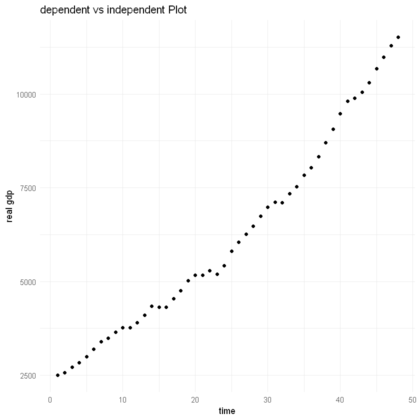
Data shows Real GDP for USA for 1960-2007

model4 <- lm(lnrgdp ~ time, data = df2)
tidy(model4)
glance(model4)

A tibble: 2 × 5
term	estimate	std.error	statistic	p.value
<chr>	<dbl>	<dbl>	<dbl>	<dbl>
(Intercept)	7.87566236	0.0097591072	807.00644	3.931863e-97
time	0.03148955	0.0003467383	90.81649	1.519344e-53

A tibble: 1 × 12
r.squared	adj.r.squared	sigma	statistic	p.value	df	logLik	AIC	BIC	deviance	df.residual	nobs
<dbl>	<dbl>	<dbl>	<dbl>	<dbl>	<dbl>	<dbl>	<dbl>	<dbl>	<dbl>	<int>	<int>
0.9944536	0.994333	0.03327965	8247.634	1.519344e-53	1	96.24722	-186.4944	-180.8808	0.05094662	46	48

Time Coefficient: Real GDP increases at raate 3.15% per year

Intercept result: exp(7.87) = 2632.27 is the beginning value of real GDP at the beginning of 1960

compound interest: $\beta_2 = \ln(1+r)$. r = exp($\beta_2$)-1, r = 3.2%

Compare it with linear model#

\[ RGDP_t = \beta_0 + \beta_1 \text{time} + u_t \]

model5 <- lm(rgdp ~ time, data = df2)
tidy(model5)
glance(model5)

A tibble: 2 × 5
term	estimate	std.error	statistic	p.value
<chr>	<dbl>	<dbl>	<dbl>	<dbl>
(Intercept)	1664.2176	131.998983	12.60781	1.570394e-16
time	186.9939	4.689886	39.87174	2.523710e-37

A tibble: 1 × 12
r.squared	adj.r.squared	sigma	statistic	p.value	df	logLik	AIC	BIC	deviance	df.residual	nobs
<dbl>	<dbl>	<dbl>	<dbl>	<dbl>	<dbl>	<dbl>	<dbl>	<dbl>	<dbl>	<int>	<int>
0.9718784	0.9712671	450.1314	1589.756	2.52371e-37	1	-360.3455	726.691	732.3046	9320439	46	48

Time coefficient: real gdp increases by $187 billion per year showing positive trend

df2$residuals <- residuals(model5)
df2$fitted_values <- fitted(model5)

ggplot(df2, aes(x = time, y = rgdp)) +
  geom_point() +
  labs(title = "dependent vs independent Plot",
       x = "time",
       y = "real gdp") +
  theme_minimal()

_images/26b526b9c3268dc0012a3fbf4fde6d59e53a9407d352de995b62c627a1907463.png

Lin-LOg model#

\[ Y_i = \beta_0 + \beta_1 \ln X_i + u_i \]

df3 <- read_excel("data/Table2_8.xls")
head(df3,3)
tail(df3,3)

A tibble: 3 × 6
fdho	expend	sfdho	lnexpend	expend_rec	expend2
<dbl>	<dbl>	<dbl>	<dbl>	<dbl>	<dbl>
6475	40516.75	0.15981045	10.609470	2.468115e-05	1641607040
3146	33540.50	0.09379705	10.420509	2.981470e-05	1124965120
1632	5181.85	0.31494543	8.552917	1.929813e-04	26851570

A tibble: 3 × 6
fdho	expend	sfdho	lnexpend	expend_rec	expend2
<dbl>	<dbl>	<dbl>	<dbl>	<dbl>	<dbl>
5811	31922.20	0.1820363	10.371057	3.132616e-05	1019026816
4594	25357.25	0.1811711	10.140820	3.943645e-05	642990144
2108	7313.60	0.2882302	8.897491	1.367316e-04	53488748

Engel expenditure function theory: the total expenditure that is devoted to food tends to increase in arithmetic progression as total expenditure increases in geometric proportion.
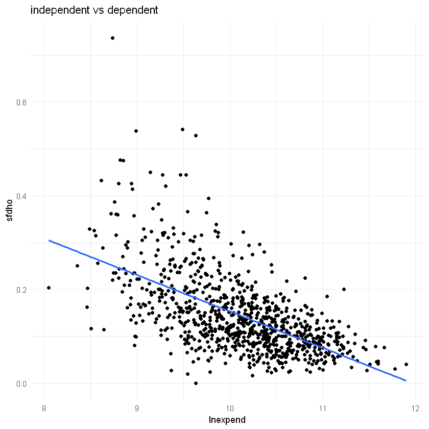
In other words: share of expenditure on food decreases as total expenditure increases

Expend: total household expenditure
SFDHO: share of food expenditure
869 US households in 1995

model6 <- lm(sfdho ~ lnexpend, data = df3)
tidy(model6)
glance(model6)

A tibble: 2 × 5
term	estimate	std.error	statistic	p.value
<chr>	<dbl>	<dbl>	<dbl>	<dbl>
(Intercept)	0.93038679	0.036366542	25.58359	5.360528e-108
lnexpend	-0.07773725	0.003590929	-21.64823	2.011079e-83

A tibble: 1 × 12
r.squared	adj.r.squared	sigma	statistic	p.value	df	logLik	AIC	BIC	deviance	df.residual	nobs
<dbl>	<dbl>	<dbl>	<dbl>	<dbl>	<dbl>	<dbl>	<dbl>	<dbl>	<dbl>	<int>	<int>
0.3508757	0.350127	0.06875045	468.6456	2.011079e-83	1	1094.493	-2182.986	-2168.684	4.097984	867	869

lnexpend coefficient: -0.08:
if expenditure increases by 1%, on average, sfhdo decreases by 0.0008 units
if expenditure increases by 100%, on average, sdfho decreases by 0.08 units

df3$residuals <- residuals(model6)
df3$fitted_values <- fitted(model6)

ggplot(df3, aes(x = lnexpend, y = sfdho)) +
  geom_point() +
  geom_smooth(method = 'lm',formula = y ~ x, se = FALSE) +
  labs(title = "independent vs dependent",
       x = "lnexpend",
       y = "sfdho") +
  theme_minimal()

_images/4c17861c950b3afea2d65680fe6e9aa1d638a218c6ac9a4af5dd400cef818031.png

Reciprocol models#

\[ Y_i = \beta_0 + \beta_1 \left(\frac{1}{X_i}\right) + u_i \]

Note: $$ \frac{dY_i}{dX_i} = -\beta_1\left(\frac{1}{X_i}^2\right) $$

model7 <- lm(sfdho ~ I(1/expend), data = df3)
tidy(model7)
glance(model7)

A tibble: 2 × 5
term	estimate	std.error	statistic	p.value
<chr>	<dbl>	<dbl>	<dbl>	<dbl>
(Intercept)	7.726305e-02	0.004011685	19.2595	4.376382e-69
I(1/expend)	1.331338e+03	63.957133553	20.8161	2.303454e-78

A tibble: 1 × 12
r.squared	adj.r.squared	sigma	statistic	p.value	df	logLik	AIC	BIC	deviance	df.residual	nobs
<dbl>	<dbl>	<dbl>	<dbl>	<dbl>	<dbl>	<dbl>	<dbl>	<dbl>	<dbl>	<int>	<int>
0.3332359	0.3324669	0.06967833	433.31	2.303454e-78	1	1082.843	-2159.686	-2145.384	4.209346	867	869

Intercept coeff: if expend increases indefinitely, sfdho will equal 8% or 0.08

slope coeff: positive slope, rate of change of sfdho with respect to expenditure is negative

ggplot(df3, aes(x = expend, y = sfdho)) +
  geom_point() +
  labs(title = "independent vs dependent",
       x = "expend",
       y = "sfdho") +
  theme_minimal()

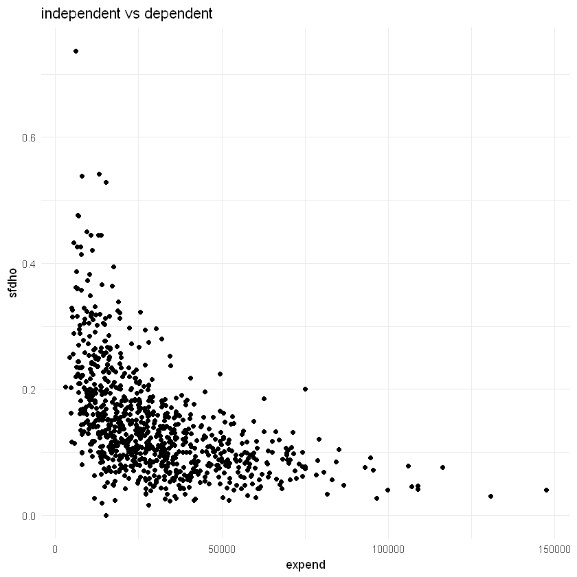
_images/6357af8ebd6fe9c0b3315731264ec220d5bc77e2738a7b2063d20cd0d7129814.png

lin-log model performed better than reciprocol model based on $R^2$, both have same dependent variable so we can compare using it

summary(model6)$r.squared
summary(model7)$r.squared

0.350875735484601

0.333235927711165

Polynomial regression model#

\[ RGDP_t = \beta_0 + \beta_1 \text{time} + \beta_2 \text{time}^2 + u_t\]

model8 <- lm(rgdp ~ time + I(time^2), data = df2)
tidy(model8)
glance(model8)

A tibble: 3 × 5
term	estimate	std.error	statistic	p.value
<chr>	<dbl>	<dbl>	<dbl>	<dbl>
(Intercept)	2651.380622	69.4908403	38.15439	6.449733e-36
time	68.534362	6.5421140	10.47587	1.187953e-13
I(time^2)	2.417542	0.1294432	18.67647	7.969017e-23

A tibble: 1 × 12
r.squared	adj.r.squared	sigma	statistic	p.value	df	logLik	AIC	BIC	deviance	df.residual	nobs
<dbl>	<dbl>	<dbl>	<dbl>	<dbl>	<dbl>	<dbl>	<dbl>	<dbl>	<dbl>	<int>	<int>
0.9967866	0.9966438	153.8419	6979.431	8.066871e-57	2	-308.2845	624.5691	632.0539	1065030	45	48

\[ \frac{dRGDP}{dtime} = \beta_1 + 2\beta_2\text{time} = 68.53 + 4.84 \text{time} \]

The rate of change of RGDP increases with an increasing rate
unlike the linear model that showed constant rate $187

Log-lin model with quadratic trend#

\[ \ln RGDP_t = \beta_0 + \beta_1 \text{time} + \beta_2 \text{time}^2 + u_t\]

\[\frac{d \ln RGDP}{dtime} = \beta_1 + 2\beta_2\text{time} = 0.0365 - 0.0002\text{time}\]

The model increases with a decreasing rate
unlike the quadratic RGDP model (model 8)

model9 <- lm(lnrgdp ~ time + I(time^2), data = df2)
tidy(model9)
glance(model9)

A tibble: 3 × 5
term	estimate	std.error	statistic	p.value
<chr>	<dbl>	<dbl>	<dbl>	<dbl>
(Intercept)	7.8334797935	1.275348e-02	614.223018	6.228568e-90
time	0.0365514617	1.200658e-03	30.442868	1.147864e-31
I(time^2)	-0.0001033042	2.375639e-05	-4.348483	7.756188e-05

A tibble: 1 × 12
r.squared	adj.r.squared	sigma	statistic	p.value	df	logLik	AIC	BIC	deviance	df.residual	nobs
<dbl>	<dbl>	<dbl>	<dbl>	<dbl>	<dbl>	<dbl>	<dbl>	<dbl>	<dbl>	<int>	<int>
0.9960946	0.9959211	0.02823421	5738.809	6.492039e-55	2	104.6665	-201.333	-193.8482	0.03587268	45	48

rate of growth of RGDP decreases at rate 0.0002 per unit of time

Comparing linear and log-log (log-linear) models#

compare_models <- function(df, dependent_var, independent_vars) {
  library(dplyr)
  library(broom)
  
  # Step 1: Compute the geometric mean (GM) of the dependent variable
  geom_mean <- exp(mean(log(df[[dependent_var]])))
  
  # Step 2: Transform the dependent variable
  df <- df %>%
    mutate(transformed_output = .[[dependent_var]] / geom_mean,
           log_output = log(transformed_output))
  
  # Create formula strings for the models
  independent_vars_formula <- paste(independent_vars, collapse = " + ")
  linear_formula <- as.formula(paste("transformed_output ~", independent_vars_formula))
  log_linear_formula <- as.formula(paste("log_output ~", paste("log(", independent_vars, ")", collapse = " + ")))
  
  # Step 3: Estimate the linear model using transformed_output
  linear_model <- lm(linear_formula, data = df)
  linear_model_tidy <- tidy(linear_model)
  linear_model_rss <- sum(residuals(linear_model)^2)
  
  # Step 4: Estimate the log-linear model using log_output
  log_linear_model <- lm(log_linear_formula, data = df)
  log_linear_model_tidy <- tidy(log_linear_model)
  log_linear_model_rss <- sum(residuals(log_linear_model)^2)
  
  # Ensure residuals sum of squares matches expected values by directly comparing them
  rss1 <- sum((df$transformed_output - predict(linear_model))^2)
  rss2 <- sum((df$log_output - predict(log_linear_model))^2)
  
 # Number of observations
  n <- nrow(df)
  
  # Compute the likelihood ratio test statistic
  lambda <- (n / 2) * log(rss1 / rss2)
  
  # Compute the p-value from the chi-square distribution with 1 degree of freedom
  p_value <- pchisq(lambda, df = 1,)
  
  # Print results
  print(linear_model_tidy)
  print(log_linear_model_tidy)
  
  # Compare RSS
  print(paste("RSS for linear model:", rss1))
  print(paste("RSS for log-linear model:", rss2))
  print(paste("Lambda (test statistic):", lambda))
  print(paste("P-value:", p_value))
  
  return(list(
    linear_model = linear_model,
    log_linear_model = log_linear_model,
    linear_model_rss = rss1,
    log_linear_model_rss = rss2,
    lambda = lambda,
    p_value = p_value
  ))
}

compare_models(df, "output", c("labor", "capital"))

# A tibble: 3 × 5
  term           estimate    std.error statistic  p.value
  <chr>             <dbl>        <dbl>     <dbl>    <dbl>
1 (Intercept) 0.0103      0.0549           0.187 8.53e- 1
2 labor       0.00000211  0.000000310      6.80  1.50e- 8
3 capital     0.000000437 0.0000000429    10.2   1.43e-13
# A tibble: 3 × 5
  term         estimate std.error statistic  p.value
  <chr>           <dbl>     <dbl>     <dbl>    <dbl>
1 (Intercept)   -13.1      0.396     -32.9  1.30e-34
2 log(labor)      0.468    0.0989      4.73 1.98e- 5
3 log(capital)    0.521    0.0969      5.38 2.18e- 6
[1] "RSS for linear model: 3.67211242597136"
[1] "RSS for log-linear model: 3.41552013886784"
[1] "Lambda (test statistic): 1.84715109633792"
[1] "P-value: 0.825884897403209"

$linear_model

Call:
lm(formula = linear_formula, data = df)

Coefficients:
(Intercept)        labor      capital  
  1.026e-02    2.107e-06    4.369e-07  


$log_linear_model

Call:
lm(formula = log_linear_formula, data = df)

Coefficients:
 (Intercept)    log(labor)  log(capital)  
    -13.0538        0.4683        0.5213  


$linear_model_rss
[1] 3.672112

$log_linear_model_rss
[1] 3.41552

$lambda
[1] 1.847151

$p_value
[1] 0.8258849

Regression on standardized variables#

standardize_variables <- function(df, dependent_var, independent_vars) {
  df[[dependent_var]] <- scale(df[[dependent_var]], center = TRUE, scale = TRUE)
  
  for (var in independent_vars) {
    df[[var]] <- scale(df[[var]], center = TRUE, scale = TRUE)
  }
  
  return(df)
}

df_standardized <- standardize_variables(df, "output", c("labor", "capital"))

model10 <- lm(output ~ labor + capital, data = df_standardized)
tidy(model10)
glance(model10)

A tibble: 3 × 5
term	estimate	std.error	statistic	p.value
<chr>	<dbl>	<dbl>	<dbl>	<dbl>
(Intercept)	2.433157e-17	0.01966566	1.237262e-15	1.000000e+00
labor	4.023881e-01	0.05918546	6.798766e+00	1.496564e-08
capital	6.021852e-01	0.05918546	1.017455e+01	1.433023e-13

A tibble: 1 × 12
r.squared	adj.r.squared	sigma	statistic	p.value	df	logLik	AIC	BIC	deviance	df.residual	nobs
<dbl>	<dbl>	<dbl>	<dbl>	<dbl>	<dbl>	<dbl>	<dbl>	<dbl>	<dbl>	<int>	<int>
0.9810653	0.9802763	0.1404409	1243.514	4.510314e-42	2	29.29145	-50.58289	-42.85559	0.9467354	48	51

intercept = tidy(model10)[[1,2]]

ifelse(intercept < .Machine$double.eps,
                 paste(intercept, "is almost zero"),
                 paste(intercept, "is not almost zero"))

'2.43315712814819e-17 is almost zero'

labor coefficient: if labor increases by one standard deviation unit, average value of output goes up by about 0.40 standard deviation units, cetris paribus

capital coefficient: if labor increases by one standard deviation unit, average value of output goes up by about 0.60 standard deviation units, cetris paribus

Note: same $R^2, t, F$
does not mean that capital is more important than labor

Regression through the origin: zero intercept model#

capital asset price model (CAPM)#

\begin{align} (ER_i-r_f) &= \beta_i(ER_m-r_f)\ ER_i &= \text{expected rate of return on security}\ ER_m &= \text{expected rate of return on market portfolio}\ r_f &= \text{risk free rate of return} \ \beta_i &= \text{systematic risk} \end{align}

To estimate

\[ (R_i-r_f) = \beta_i(R_m-r_f) + u_i\]

Where $R_i, R_m$ are observed rates of return

Let

\begin{align} Y_i = R_i - r_f = \text{rate of return on security i in excess of the risk-free rate of return}\ X_i = R_m - r_f = \text{rate of return on market in excess of the risk-free rate of return} \end{align}

\[ Y_i = \beta X_i + u_i \]

df4 <- read_excel("data/Table2_15.xls")
head(df4,3)
dim(df4)

A tibble: 3 × 2
y	x
<dbl>	<dbl>
6.080228	7.263448
-0.924186	6.339896
-3.286174	-9.285217

240
2

model11 <- lm(y ~ 0 + x, data = df4)
model12 <- lm(y ~ x, data = df4)

tidy(model11)
glance(model11)

A tibble: 1 × 5
term	estimate	std.error	statistic	p.value
<chr>	<dbl>	<dbl>	<dbl>	<dbl>
x	1.155512	0.07439562	15.532	4.405444e-38

A tibble: 1 × 12
r.squared	adj.r.squared	sigma	statistic	p.value	df	logLik	AIC	BIC	deviance	df.residual	nobs
<dbl>	<dbl>	<dbl>	<dbl>	<dbl>	<dbl>	<dbl>	<dbl>	<dbl>	<dbl>	<int>	<int>
0.5023352	0.5002529	5.548786	NA	NA	NA	-751.3032	1506.606	1513.568	7358.578	239	240

Raw $R^2$: 0.5
proportion of variation around the origin

tidy(model12)
glance(model12)

A tibble: 2 × 5
term	estimate	std.error	statistic	p.value
<chr>	<dbl>	<dbl>	<dbl>	<dbl>
(Intercept)	-0.4474811	0.36294281	-1.232925	2.188203e-01
x	1.1711284	0.07538643	15.535004	4.752177e-38

A tibble: 1 × 12
r.squared	adj.r.squared	sigma	statistic	p.value	df	logLik	AIC	BIC	deviance	df.residual	nobs
<dbl>	<dbl>	<dbl>	<dbl>	<dbl>	<dbl>	<dbl>	<dbl>	<dbl>	<dbl>	<int>	<int>
0.5034802	0.501394	5.542759	241.3363	4.752177e-38	1	-750.5392	1507.078	1517.52	7311.877	238	240

as.numeric(tidy(model12)[[1,'p.value']])

0.218820272828606

Intercept: not significant, use model11 instead

Measures of goodness of fit#

print(paste("R Squared: ",glance(model12)$r.squared))

[1] "R Squared:  0.503480169868958"

print(paste("Adjusted R Squared: ",glance(model12)$adj.r.squared))

[1] "Adjusted R Squared:  0.501393952095298"

print(paste("Akaike's Information Criteria: ", glance(model12)$AIC))

[1] "Akaike's Information Criteria:  1507.07843469119"

print(paste("Schwarz’s Information Criterion:",glance(model12)$BIC))

[1] "Schwarz’s Information Criterion: 1517.52035146121"

print(paste("Log Likelihood:",glance(model12)$logLik))

[1] "Log Likelihood: -750.539217345594"

colnames(glance(model12))

'r.squared'
'adj.r.squared'
'sigma'
'statistic'
'p.value'
'df'
'logLik'
'AIC'
'BIC'
'deviance'
'df.residual'
'nobs'

Exercises#

2.1#

Consider the following production function, known in the literature as the transcendental production function (TPF)

\[\begin{split} Q_i = B_1L_i^{\beta_2} K_i^{\beta_3} e^{\beta_4L_i+ \beta_5K_i} \\ \end{split}\]

$\text{where Q, L, and K represent output, labor, and capital, respectively}$

a#

How would you linearize this function?

\[ \ln Q_i = \ln \beta_1 + \beta_2 \ln L_i + \beta_3 \ln K_i + \beta_4 L_i + \beta_5 K_i \]

b#

What is the interpretation of the various coefficients in the TPF?

$\beta_1$: y intercept
labor: elasticity = $\beta_2 + \beta_4 L_i$
capital:: elasticity = $\beta_3 + \beta_5 K_i$

c#

Given the data in Table 2.1, estimate the parameters of the TPF

df5 <- read_excel("G:/Datasets/Econometrics BY Example/Excel/Table2_1.xls")
head(df5)

A tibble: 6 × 12
obs	output	labor	capital	lnoutput	lnlabor	lncapital	lnoutlab	lncaplab	outputstar	capitalstar	laborstar
<dbl>	<dbl>	<dbl>	<dbl>	<dbl>	<dbl>	<dbl>	<dbl>	<dbl>	<dbl>	<dbl>	<dbl>
1	38372840	424471	2689076	17.46286	12.958599	14.80471	4.504261	1.846109	-0.1079874	0.06368887	0.1343891
2	1805427	19895	57997	14.40631	9.898224	10.96815	4.508084	1.069923	-0.9230660	-0.90551400	-0.9410533
3	23736129	206893	2308272	16.98251	12.239957	14.65201	4.742552	2.412053	-0.4342360	-0.07658678	-0.4439759
4	26981983	304055	1376235	17.11068	12.624964	14.13486	4.485716	1.509898	-0.3618868	-0.41991854	-0.1857003
5	217546032	1809756	13554116	19.19792	14.408703	16.42220	4.789218	2.013498	3.8857391	4.06601191	3.8167481
6	19462751	180366	1790751	16.78401	12.102743	14.39815	4.681270	2.295402	-0.5294886	-0.26722449	-0.5144899

model13 <- lm(lnoutput ~ lnlabor + lncapital + labor + capital, data = df5)
tidy(model13)
glance(model13)

A tibble: 5 × 5
term	estimate	std.error	statistic	p.value
<chr>	<dbl>	<dbl>	<dbl>	<dbl>
(Intercept)	3.949841e+00	5.660371e-01	6.9780608	9.829494e-09
lnlabor	5.208141e-01	1.347469e-01	3.8651277	3.465680e-04
lncapital	4.717828e-01	1.231899e-01	3.8297200	3.865161e-04
labor	-2.519414e-07	4.201003e-07	-0.5997173	5.516375e-01
capital	3.552743e-08	5.299532e-08	0.6703880	5.059624e-01

A tibble: 1 × 12
r.squared	adj.r.squared	sigma	statistic	p.value	df	logLik	AIC	BIC	deviance	df.residual	nobs
<dbl>	<dbl>	<dbl>	<dbl>	<dbl>	<dbl>	<dbl>	<dbl>	<dbl>	<dbl>	<int>	<int>
0.9645228	0.9614378	0.271165	312.6518	1.032818e-32	4	-3.17825	18.3565	29.94745	3.382401	46	51

(intercept <-exp(tidy(model13)[[1,2]]))

51.9271343254996

df5 |> 
summarize(mean_labor = mean(labor),
         mean_capital = mean(capital))

A tibble: 1 × 2
mean_labor	mean_capital
<dbl>	<dbl>
373914.5	2516181

print(paste("elasticity of labor at mean:",5.208141e-01+ -2.519414e-07*373914.5 ))

[1] "elasticity of labor at mean: 0.4266095573897"

d#

Suppose you want to test the hypothesis that B4 = B5 = 0. How would you test these hypotheses? Show the necessary calculations.

full_model <- lm(log(output) ~ log(labor) + log(capital) + labor + capital, data = df5)
restricted_model <- lm(log(output) ~ log(labor) + log(capital), data = df5)


(anova_result <- anova(restricted_model, full_model))

f_statistic <- anova_result$F[2]
p_value <- anova_result$`Pr(>F)`[2]

cat("F-statistic:", f_statistic, "\n")
cat("P-value:", p_value, "\n")

if (p_value < 0.05) {
  cat("Reject the null hypothesis: There is evidence that at least one of beta_4 or beta_5 is not equal to zero.\n")
} else {
  cat("Fail to reject the null hypothesis: There is no evidence that beta_4 or beta_5 are different from zero.\n")
}

A anova: 2 × 6
	Res.Df	RSS	Df	Sum of Sq	F	Pr(>F)
	<dbl>	<dbl>	<dbl>	<dbl>	<dbl>	<dbl>
1	48	3.415520	NA	NA	NA	NA
2	46	3.382404	2	0.03311649	0.2251887	0.7992404

F-statistic: 0.2251887 
P-value: 0.7992404 
Fail to reject the null hypothesis: There is no evidence that beta_4 or beta_5 are different from zero.

e#

How would you compute the output-labor and output capital elasticities for this model? Are they constant or variable?

variable