6. Autocorrelation

6. Autocorrelation#

suppressPackageStartupMessages({
  library(tidyverse)
  library(tidymodels)
  library(readxl)
  library(multcomp)
  library(car)
  library(lmtest)
  library(sandwich)
})

US Consumption function 1947-2000#

df <- read_excel("data/Table6_1.xls")
head(df)

A tibble: 6 × 24
year	consumption	income	wealth	interest	lnconsump	lndpi	lnwealth	dlnconsump	dlndpi	⋯	rlnwealth	rinterest	dconsump	dincome	dwealth	rconsump	rincome	rwealth	rinterest2	time
<dbl>	<dbl>	<dbl>	<dbl>	<dbl>	<dbl>	<dbl>	<dbl>	<dbl>	<dbl>	⋯	<dbl>	<dbl>	<dbl>	<dbl>	<dbl>	<dbl>	<dbl>	<dbl>	<dbl>	<dbl>
21916	976.4	1035.2	5166.815	-10.350940	6.883873	6.942350	8.550012	NA	NA	⋯	NA	NA	NA	NA	NA	NA	NA	NA	NA	1
21916	998.1	1090.0	5280.757	-4.719804	6.905853	6.993933	8.571825	0.02198076	0.051583290	⋯	5.795887	-1.35915709	21.69995	54.800049	113.9419	704.3560	778.5664	3726.352	-1.60578680	2
21916	1025.3	1095.6	5607.351	1.044063	6.932741	6.999057	8.631834	0.02688742	0.005124092	⋯	5.848814	2.57644486	27.20007	5.599976	326.5942	725.0278	767.6801	4018.668	2.46398711	3
21916	1090.9	1192.7	5759.515	0.407346	6.994758	7.083975	8.658608	0.06201744	0.084917545	⋯	5.856105	0.06836937	65.59998	97.099976	152.1641	782.4448	863.0954	4072.578	0.09324604	4
21916	1107.1	1227.0	6086.056	-5.283152	7.009499	7.112328	8.713756	0.01474094	0.028352737	⋯	5.902559	-5.41540527	16.19995	34.300049	326.5410	778.9094	868.1835	4353.341	-5.40569973	5
21916	1142.4	1266.8	6243.864	-0.277011	7.040886	7.144249	8.739354	0.03138733	0.031921864	⋯	5.910253	1.43827367	35.30005	39.800049	157.8076	809.3358	897.6646	4412.911	1.31239307	6

colnames(df)

'year'
'consumption'
'income'
'wealth'
'interest'
'lnconsump'
'lndpi'
'lnwealth'
'dlnconsump'
'dlndpi'
'dlnwealth'
'dinterest'
'rlnconsump'
'rlndpi'
'rlnwealth'
'rinterest'
'dconsump'
'dincome'
'dwealth'
'rconsump'
'rincome'
'rwealth'
'rinterest2'
'time'

\[ \ln C_T = \beta_1 + \beta_2 \ln DPI_t + \beta_3 \ln W_t + \beta_4 R_t + u_t \]

real consumption expenditure (C),
real (after tax) disposable personal income (DPI),
real wealth (W)
and real interest rate (R)

model <- lm(lnconsump ~ lndpi + lnwealth +  interest, data =df)
tidy(model)
glance(model)

A tibble: 4 × 5
term	estimate	std.error	statistic	p.value
<chr>	<dbl>	<dbl>	<dbl>	<dbl>
(Intercept)	-0.467712044	0.0427779986	-10.933472	7.330410e-15
lndpi	0.804872759	0.0174978490	45.998383	1.376236e-42
lnwealth	0.201270215	0.0175925850	11.440628	1.433544e-15
interest	-0.002689061	0.0007619294	-3.529279	9.046458e-04

A tibble: 1 × 12
r.squared	adj.r.squared	sigma	statistic	p.value	df	logLik	AIC	BIC	deviance	df.residual	nobs
<dbl>	<dbl>	<dbl>	<dbl>	<dbl>	<dbl>	<dbl>	<dbl>	<dbl>	<dbl>	<int>	<int>
0.9995597	0.9995332	0.01193375	37832.66	7.120776e-84	3	164.588	-319.1761	-309.2312	0.007120721	50	54

if real personal disposal income goes up by 1%, mean real consumption expenditure goes up by about 0.8%

if real wealth goes up by 1%, mean real consumption expenditure goes up by about 0.2%,

if rate goes up by one percentage point, mean real consumption expenditure goes down by about 0.26%

\(R^2\) indicating spurious correlation

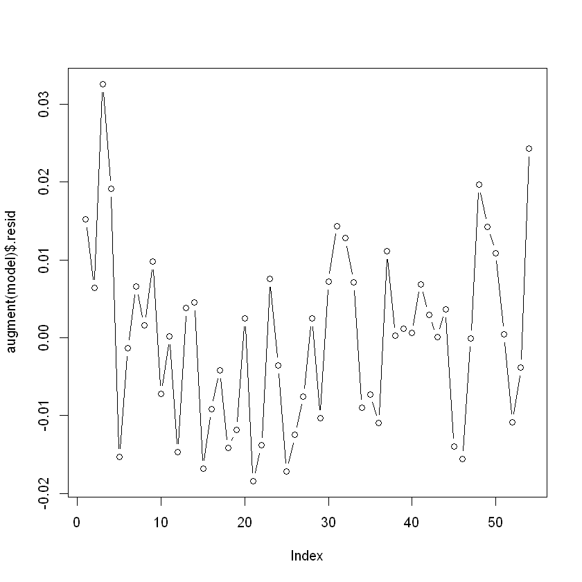
Tests of autocorrelation#

plot(augment(model)$.resid, type = 'b')

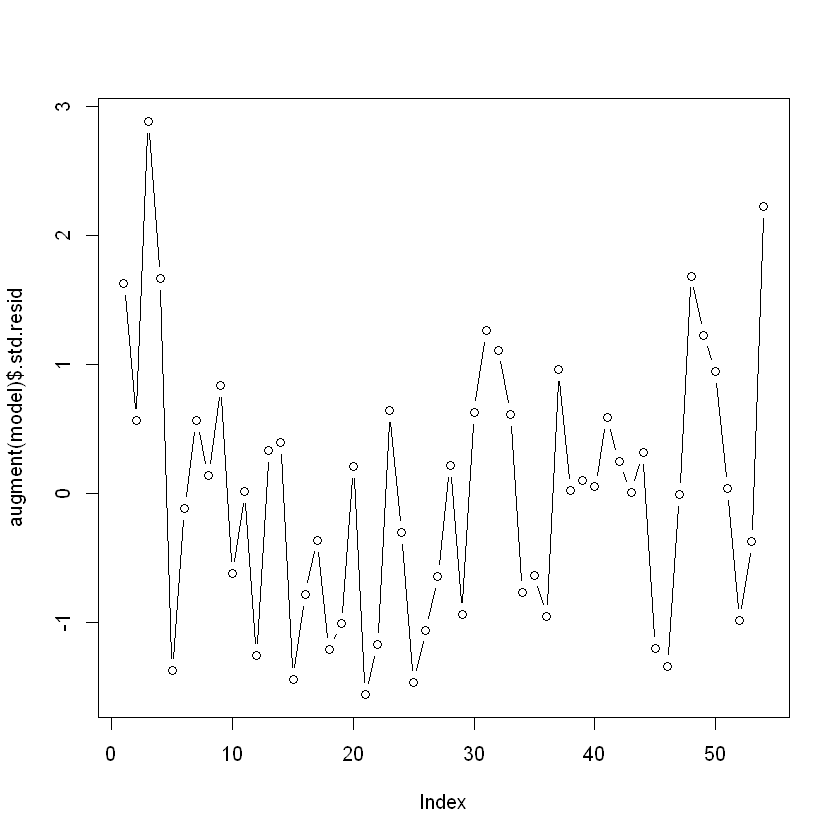
_images/6a3ba80af82312e4d24489d3148c7d9db2a07af2c8a69d02540a3db91cf090d2.png

plot(augment(model)$.std.resid, type = 'b')

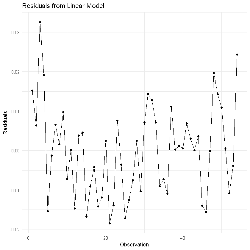
_images/f15753b446692c94bf65c4b439d864d5658cdbd5b8193a5142ee9c87b60b627a.png

augmented_data <- augment(model)

ggplot(augmented_data, aes(x = seq_along(.resid), y = .resid)) +
  geom_line() +
  geom_point() +
  labs(title = "Residuals from Linear Model",
       x = "Observation",
       y = "Residuals") +
  theme_minimal()

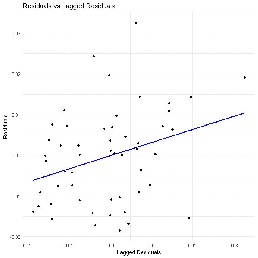
_images/58ddc665f281bc726051c39b610cd903b43ab2767b383fb9174bc4489cc2947b.png

augmented_data <- augmented_data %>%
  mutate(lagged_resid = lag(.resid))

# remove first row of NA lagged residual
augmented_data <- augmented_data %>%
  filter(!is.na(lagged_resid))

correlation <- cor(augmented_data$.resid, augmented_data$lagged_resid)


ggplot(augmented_data, aes(x = lagged_resid, y = .resid)) +
  geom_point() +
  geom_smooth(method = "lm",formula = 'y ~ x', se = FALSE, color = "blue") +
  labs(title = "Residuals vs Lagged Residuals",
       x = "Lagged Residuals",
       y = "Residuals") +
  theme_minimal()

_images/26df109911864c9537523ff68120fb0af2fc9593647507efe0a411f94b8e7a09.png

Durbin watson test#

must have an intercept term

durbinWatsonTest(model)

 lag Autocorrelation D-W Statistic p-value
   1       0.2977555      1.289232       0
 Alternative hypothesis: rho != 0

durbinWatsonTest(model, max.lag = 3)

 lag Autocorrelation D-W Statistic p-value
   1      0.29775555      1.289232   0.000
   2     -0.02840613      1.933710   0.694
   3      0.01631809      1.678649   0.262
 Alternative hypothesis: rho[lag] != 0

dwtest(model)

	Durbin-Watson test

data:  model
DW = 1.2892, p-value = 0.0009445
alternative hypothesis: true autocorrelation is greater than 0

Bruech Godfrey general test#

bgtest(model, order = 1)

	Breusch-Godfrey test for serial correlation of order up to 1

data:  model
LM test = 5.312, df = 1, p-value = 0.02118

bgtest(model, order = 2)

	Breusch-Godfrey test for serial correlation of order up to 2

data:  model
LM test = 6.4472, df = 2, p-value = 0.03981

bgtest(model, order = 3)

	Breusch-Godfrey test for serial correlation of order up to 3

data:  model
LM test = 6.6573, df = 3, p-value = 0.08366

AR(2) is significant, residuals follow AR(2)

Remedial measures#

First Difference#

\[ u_t - \rho u_{t-1} = v_t \]

\begin{align} \ln C_t- \rho \ln C_{t-1}&= \beta_{1(1- \rho)} \ &+ \beta_2 (\ln DPI_t - \rho \ln DPI_{t-1})\ &+ \beta_3 (\ln W_t - \rho \ln W_{t-1}) \ &+ \beta_4 (R_t - R_{t-1}) \ &+ (u_t - \rho u_{t-1}) \end{align}

if \(\rho\) = 1

\[ \Delta \ln C_t = \beta_2 \Delta \ln DPI_t + \beta_3 \Delta \ln W_t + \beta_4 \Delta R_t + v_t \]

Called first difference transformation

model2 <- lm(diff(lnconsump) ~ 0 +diff(lndpi) + diff(lnwealth) +  diff(interest), data =df)
tidy(model2)
glance(model2)

A tibble: 3 × 5
term	estimate	std.error	statistic	p.value
<chr>	<dbl>	<dbl>	<dbl>	<dbl>
diff(lndpi)	0.8489940413	0.0515376309	16.4732842	7.667028e-22
diff(lnwealth)	0.1063549555	0.0368543147	2.8858210	5.749199e-03
diff(interest)	0.0006530138	0.0008260853	0.7904919	4.329740e-01

A tibble: 1 × 12
r.squared	adj.r.squared	sigma	statistic	p.value	df	logLik	AIC	BIC	deviance	df.residual	nobs
<dbl>	<dbl>	<dbl>	<dbl>	<dbl>	<dbl>	<dbl>	<dbl>	<dbl>	<dbl>	<int>	<int>
0.9236527	0.9190718	0.0111335	201.6339	6.473553e-28	3	164.7236	-321.4472	-313.5661	0.006197738	50	53

bgtest(model2)

	Breusch-Godfrey test for serial correlation of order up to 1

data:  model2
LM test = 0.86275, df = 1, p-value = 0.353

dwtest(model2)

	Durbin-Watson test

data:  model2
DW = 2.0265, p-value = 0.547
alternative hypothesis: true autocorrelation is greater than 0

durbinWatsonTest(model2)

 lag Autocorrelation D-W Statistic p-value
   1      -0.1150018      2.026542   0.916
 Alternative hypothesis: rho != 0

feasible generalized least squares (FGLS)#

residuals = augment(model)$.resid
residuals

0.0151792320906274
0.00639409190557938
0.0325786316647871
0.0191471920745867
-0.0153337901242683
-0.00132990098127195
0.00653719274943132
0.00162048925147751
0.00975015218633235
-0.00722925871798008
0.000174758857319546
-0.0146975939327243
0.00380689173579718
0.00454249958702402
-0.0167822153758674
-0.0091399779495811
-0.00422252846219351
-0.014143908709439
-0.011875949295832
0.00245712248775831
-0.0184412867267767
-0.0138427704324453
0.00757496364792853
-0.00357671809715665
-0.0171562076207774
-0.0124861952550575
-0.00754242394929072
0.00245643437586018
-0.0102882063980623
0.00718617423785339
0.0143585227051846
0.0127678086817866
0.0070919535900682
-0.00903155158175295
-0.00726634215564381
-0.0109670199434095
0.0110890173466256
0.000254097439515988
0.00116108304687401
0.000586076244815104
0.00687811518401915
0.00293814373603141
8.79859166129648e-05
0.00366504301640092
-0.0140024869709681
-0.0155797023743123
-0.00012753645438579
0.0196279528980181
0.0142734120216019
0.0108911843032331
0.000420259520168997
-0.0108587536823013
-0.00387038232170589
0.024296225009854

rho <- coef(lm(residuals ~ 0 + lag(residuals)))
rho

lag(residuals): 0.324670692527429

dwtest(model)

	Durbin-Watson test

data:  model
DW = 1.2892, p-value = 0.0009445
alternative hypothesis: true autocorrelation is greater than 0

durbinWatsonTest(model)

 lag Autocorrelation D-W Statistic p-value
   1       0.2977555      1.289232   0.004
 Alternative hypothesis: rho != 0

rho2 = 1 - (1.289232/2) 
rho2

0.355384

fgls_model <- lm(I(lnconsump-rho*lag(lnconsump)) ~ I(lndpi-rho*lag(lndpi)) + 
                 I(lnwealth-rho*lag(lnwealth)) + I(interest-rho*lag(interest)) , data = df)
tidy(fgls_model)
glance(fgls_model)

A tibble: 4 × 5
term	estimate	std.error	statistic	p.value
<chr>	<dbl>	<dbl>	<dbl>	<dbl>
(Intercept)	-2.797310e-01	0.033726467	-8.2941093	6.807447e-11
I(lndpi - rho * lag(lndpi))	8.187056e-01	0.021096888	38.8069362	1.878713e-38
I(lnwealth - rho * lag(lnwealth))	1.836285e-01	0.020987236	8.7495302	1.396990e-11
I(interest - rho * lag(interest))	-1.799604e-05	0.000969139	-0.0185691	9.852603e-01

A tibble: 1 × 12
r.squared	adj.r.squared	sigma	statistic	p.value	df	logLik	AIC	BIC	deviance	df.residual	nobs
<dbl>	<dbl>	<dbl>	<dbl>	<dbl>	<dbl>	<dbl>	<dbl>	<dbl>	<dbl>	<int>	<int>
0.9992348	0.999188	0.0104226	21330.12	2.542681e-76	3	168.756	-327.512	-317.6606	0.005322902	49	53

bgtest(fgls_model)

	Breusch-Godfrey test for serial correlation of order up to 1

data:  fgls_model
LM test = 2.8168, df = 1, p-value = 0.09328

dwtest(fgls_model)

	Durbin-Watson test

data:  fgls_model
DW = 1.449, p-value = 0.008542
alternative hypothesis: true autocorrelation is greater than 0

durbinWatsonTest(fgls_model)

 lag Autocorrelation D-W Statistic p-value
   1       0.2092955      1.448986   0.014
 Alternative hypothesis: rho != 0

library(dynlm)


# Create the FGLS formula
fgls_formula <- as.formula(paste("I(lnconsump - ", rho, "* lag(lnconsump)) ~ ",
                                 "I(lndpi - ", rho, "* lag(lndpi)) + ",
                                 "I(lnwealth - ", rho, "* lag(lnwealth)) + ",
                                 "I(interest - ", rho, "* lag(interest))"
))

# Fit the FGLS model using dynlm
fgls_model <- dynlm(fgls_formula, data = df)

# Tidy model coefficients
tidy(fgls_model)

# Model summary
glance(fgls_model)

Warning message:
"The `tidy()` method for objects of class `dynlm` is not maintained by the broom team, and is only supported through the `lm` tidier method. Please be cautious in interpreting and reporting broom output.

This warning is displayed once per session."

A tibble: 4 × 5
term	estimate	std.error	statistic	p.value
<chr>	<dbl>	<dbl>	<dbl>	<dbl>
(Intercept)	-2.797310e-01	0.033726467	-8.2941093	6.807447e-11
I(lndpi - 0.324670692527429 * lag(lndpi))	8.187056e-01	0.021096888	38.8069362	1.878713e-38
I(lnwealth - 0.324670692527429 * lag(lnwealth))	1.836285e-01	0.020987236	8.7495302	1.396990e-11
I(interest - 0.324670692527429 * lag(interest))	-1.799604e-05	0.000969139	-0.0185691	9.852603e-01

A tibble: 1 × 12
r.squared	adj.r.squared	sigma	statistic	p.value	df	logLik	AIC	BIC	deviance	df.residual	nobs
<dbl>	<dbl>	<dbl>	<dbl>	<dbl>	<dbl>	<dbl>	<dbl>	<dbl>	<dbl>	<int>	<int>
0.9992348	0.999188	0.0104226	21330.12	2.542681e-76	3	168.756	-327.512	-317.6606	0.005322902	49	53

library(dynlm)

# Fit the original model
model <- lm(lnconsump ~ lndpi + lnwealth + interest, data = df)

# Get residuals
residuals <- residuals(model)

# Estimate AR(2) coefficients
ar_model <- lm(residuals ~ lag(residuals, 1) + lag(residuals, 2))
rho1 <- coef(ar_model)[2]
rho2 <- coef(ar_model)[3]

# Create the FGLS formula for AR(2)
fgls_formula <- as.formula(paste("I(lnconsump - ", rho1, "* lag(lnconsump, 1) - ", rho2, "* lag(lnconsump, 2)) ~ ",
                                 "I(lndpi - ", rho1, "* lag(lndpi, 1) - ", rho2, "* lag(lndpi, 2)) + ",
                                 "I(lnwealth - ", rho1, "* lag(lnwealth, 1) - ", rho2, "* lag(lnwealth, 2)) + ",
                                 "I(interest - ", rho1, "* lag(interest, 1) - ", rho2, "* lag(interest, 2))"
))


fgls_model <- lm(fgls_formula, data = df)

tidy(fgls_model)

glance(fgls_model)

A tibble: 4 × 5
term	estimate	std.error	statistic	p.value
<chr>	<dbl>	<dbl>	<dbl>	<dbl>
(Intercept)	-0.3402025749	0.037997412	-8.9533091	8.307709e-12
I(lndpi - 0.375966677578179 * lag(lndpi, 1) - -0.159419476639279 * lag(lndpi, 2))	0.8121613433	0.019923567	40.7638520	6.679649e-39
I(lnwealth - 0.375966677578179 * lag(lnwealth, 1) - -0.159419476639279 * lag(lnwealth, 2))	0.1913213476	0.019988221	9.5717046	1.040704e-12
I(interest - 0.375966677578179 * lag(interest, 1) - -0.159419476639279 * lag(interest, 2))	-0.0007507104	0.001005589	-0.7465382	4.589834e-01

A tibble: 1 × 12
r.squared	adj.r.squared	sigma	statistic	p.value	df	logLik	AIC	BIC	deviance	df.residual	nobs
<dbl>	<dbl>	<dbl>	<dbl>	<dbl>	<dbl>	<dbl>	<dbl>	<dbl>	<dbl>	<int>	<int>
0.9993667	0.9993271	0.01078611	25247.09	9.734735e-77	3	163.8301	-317.6602	-307.904	0.005584327	48	52

Newey–West method of correcting OLS standard errors#

NeweyWest(model)

A matrix: 4 × 4 of type dbl
	(Intercept)	lndpi	lnwealth	interest
(Intercept)	1.971479e-03	2.692235e-05	-2.333159e-04	2.652791e-05
lndpi	2.692235e-05	2.628983e-04	-2.225614e-04	-6.845951e-06
lnwealth	-2.333159e-04	-2.225614e-04	2.109662e-04	2.866692e-06
interest	2.652791e-05	-6.845951e-06	2.866692e-06	6.724860e-07

Model Evaluation#

consider case of specification error

model4 <- lm(lnconsump ~ log(income) + lnwealth +  interest + lag(lnconsump), data =df)
tidy(model4)
glance(model4)

A tibble: 5 × 5
term	estimate	std.error	statistic	p.value
<chr>	<dbl>	<dbl>	<dbl>	<dbl>
(Intercept)	-0.316021364	0.0556667072	-5.6770264	7.777927e-07
log(income)	0.574833115	0.0696731710	8.2504227	9.237758e-11
lnwealth	0.150288163	0.0208376010	7.2123544	3.477275e-09
interest	-0.000675206	0.0008937643	-0.7554632	4.536624e-01
lag(lnconsump)	0.276561599	0.0804719157	3.4367468	1.225013e-03

A tibble: 1 × 12
r.squared	adj.r.squared	sigma	statistic	p.value	df	logLik	AIC	BIC	deviance	df.residual	nobs
<dbl>	<dbl>	<dbl>	<dbl>	<dbl>	<dbl>	<dbl>	<dbl>	<dbl>	<dbl>	<int>	<int>
0.9996454	0.9996159	0.01061906	33833.64	3.891148e-82	4	168.3127	-324.6254	-312.8037	0.005412694	48	53

bgtest(model4)

	Breusch-Godfrey test for serial correlation of order up to 1

data:  model4
LM test = 4.4804, df = 1, p-value = 0.03429

Exercises#

🚧 Under Construction