5. Heteroscedasticity

5. Heteroscedasticity#

suppressPackageStartupMessages({
  library(tidyverse)
  library(tidymodels)
  library(readxl)
  library(multcomp)
  library(car)
  library(lmtest)
  library(sandwich)
})

df <- read_excel("data/Table5_1.xls")
head(df)

A tibble: 6 × 10
state	abortion	religion	price	laws	funds	educ	income	picket	lnabortion
<chr>	<dbl>	<dbl>	<dbl>	<dbl>	<dbl>	<dbl>	<dbl>	<dbl>	<dbl>
MISSISSIPPI	12.4	38.0	256	0	0	64.3	14082	100	2.517696
NEW_MEXICO	17.7	44.7	332	0	0	75.1	15458	20	2.873565
UTAH	9.3	76.7	298	1	0	85.1	15573	0	2.230014
WEST_VIRGINIA	7.7	9.8	251	0	1	66.0	15598	50	2.041220
ARKANSAS	13.5	30.0	248	1	0	66.3	15635	33	2.602690
LOUISIANA	13.4	50.9	228	1	0	68.3	15931	60	2.595255

Abortion rate
State = name of the state (50 US states).
ABR = Abortion rate, number of abortions per thousand women aged 15–44 in 1992.
Religion = the percent of a state’s population that is Catholic, Southern Baptist, Evangelical, or Mormon.
Price = the average price charged in 1993 in non-hospital facilities for an abortion at 10 weeks with local anesthesia (weighted by the number of abortions performed in 1992).
Laws = a variable that takes the value of 1 if a state enforces a law that restricts a minor’s access to abortion, 0 otherwise.
Funds = a variable that takes the value of 1 if state funds are available for use to pay for an abortion under most circumstances, 0 otherwise.
Educ = the percent of a state’s population that is 25 years or older with a high school degree (or equivalent), 1990.
Income = disposable income per capita, 1992.
Picket = the percentage of respondents that reported experiencing picketing with physical contact or blocking of patients.

model <- lm(abortion ~ religion + price + laws + funds + educ + income + picket, data =df)
tidy(model)
glance(model)

A tibble: 8 × 5
term	estimate	std.error	statistic	p.value
<chr>	<dbl>	<dbl>	<dbl>	<dbl>
(Intercept)	14.283957280	1.507763e+01	0.9473609	3.488740e-01
religion	0.020070901	8.638054e-02	0.2323544	8.173913e-01
price	-0.042363106	2.222320e-02	-1.9062555	6.347505e-02
laws	-0.873101786	2.376566e+00	-0.3673795	7.151807e-01
funds	2.820003024	2.783475e+00	1.0131233	3.168024e-01
educ	-0.287255121	1.995545e-01	-1.4394818	1.574261e-01
income	0.002400682	4.551884e-04	5.2740410	4.354736e-06
picket	-0.116871214	4.217986e-02	-2.7707823	8.295326e-03

A tibble: 1 × 12
r.squared	adj.r.squared	sigma	statistic	p.value	df	logLik	AIC	BIC	deviance	df.residual	nobs
<dbl>	<dbl>	<dbl>	<dbl>	<dbl>	<dbl>	<dbl>	<dbl>	<dbl>	<dbl>	<int>	<int>
0.5774263	0.5069973	7.062582	8.198706	2.847197e-06	7	-164.3286	346.6572	363.8655	2094.962	42	50

data <-augment(model)
data <- data |> 
mutate(squared_resid = .resid^2)
data |>
ggplot(aes(x = squared_resid)) +
geom_histogram(bins  = 10)

_images/915503e53d0cd0d570b4c0fa488177504c68f4cd6d1584d5a01be48a51d0f2ce.png

ggplot(data, aes(x = .fitted, y = squared_resid))+
geom_point()

_images/ca59f4c32d44d4c5b4d89541232da5046ef3fe11c9c92e88b3ab173f5c4429d7.png

Breusch–Pagan (BP) test#

bptest(model, studentize = TRUE, data = df)

	studentized Breusch-Pagan test

data:  model
BP = 16.001, df = 7, p-value = 0.02511

White test#

white_test_result <- bptest(model, ~ religion + price + laws + funds + educ + income + picket + I(religion^2) + I(price^2) + I(laws^2) + I(funds^2) + I(educ^2) + I(income^2) + I(picket^2) +
                            religion:price + religion:laws + religion:funds + religion:educ + religion:income + 
                            religion:picket + price:laws + price:funds + price:educ + price:income + price:picket + laws:funds + 
                            laws:educ + laws:income + laws:picket + funds:educ + funds:income + funds:picket + educ:income + educ:picket + income:picket, 
                            data = df)

# Print the test results
print(white_test_result)

# Check if we reject the null hypothesis of homoscedasticity
if (white_test_result$p.value < 0.05) {
  cat("Reject the null hypothesis of homoscedasticity. The model suffers from heteroscedasticity.\n")
} else {
  cat("Do not reject the null hypothesis of homoscedasticity. The model does not suffer from heteroscedasticity.\n")
}

	studentized Breusch-Pagan test

data:  model
BP = 32.102, df = 33, p-value = 0.5116

Do not reject the null hypothesis of homoscedasticity. The model does not suffer from heteroscedasticity.

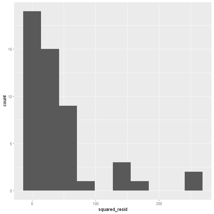
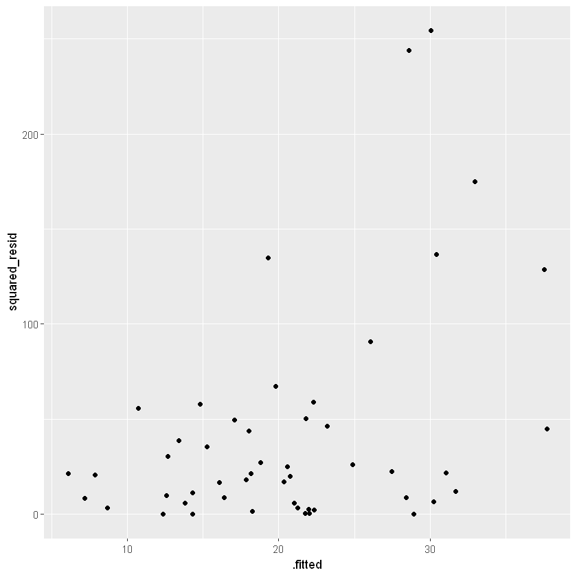
Abridged white test#

data <- augment(model)
data <- data |>
    mutate(squared_resid = .resid^2)

model2 <- lm(squared_resid ~ .fitted + I(.fitted^2), data = data)
tidy(model2)
glance(model2)

A tibble: 3 × 5
term	estimate	std.error	statistic	p.value
<chr>	<dbl>	<dbl>	<dbl>	<dbl>
(Intercept)	20.2023995	49.030794	0.4120349	0.6821871
.fitted	-1.4552665	4.759941	-0.3057321	0.7611587
I(.fitted^2)	0.1074319	0.107890	0.9957548	0.3244684

A tibble: 1 × 12
r.squared	adj.r.squared	sigma	statistic	p.value	df	logLik	AIC	BIC	deviance	df.residual	nobs
<dbl>	<dbl>	<dbl>	<dbl>	<dbl>	<dbl>	<dbl>	<dbl>	<dbl>	<dbl>	<int>	<int>
0.1930826	0.1587457	53.13374	5.623181	0.006463723	2	-268.0407	544.0813	551.7294	132690.2	47	50

p value for F = 0.006463723, we suffer from heteroscedasticity

df <- read_excel("data/Table5_1.xls")
model <- lm(abortion ~ religion + price + laws + funds + educ + income + picket, data =df)

fitted_values <- fitted(model)

df_transformed <- df

df_transformed <- df_transformed %>%
  mutate(across(where(is.numeric), ~ ./fitted_values))


model2 <- lm(abortion ~ religion + price + laws + funds + 
             educ + income + picket, data = df_transformed)
tidy(model2)
glance(model2)

A tibble: 8 × 5
term	estimate	std.error	statistic	p.value
<chr>	<dbl>	<dbl>	<dbl>	<dbl>
(Intercept)	0.8973606106	0.786093091	1.14154497	0.2601101
religion	0.0480774987	0.075204771	0.63928788	0.5261073
price	-0.0134525362	0.037889433	-0.35504717	0.7243310
laws	-0.5879502539	2.179388159	-0.26977767	0.7886524
funds	0.1956207473	3.709311583	0.05273775	0.9581909
educ	0.0288684135	0.174382545	0.16554646	0.8693082
income	0.0000652594	0.002101188	0.03105833	0.9753701
picket	0.0223771929	0.084639962	0.26438094	0.7927795

A tibble: 1 × 12
r.squared	adj.r.squared	sigma	statistic	p.value	df	logLik	AIC	BIC	deviance	df.residual	nobs
<dbl>	<dbl>	<dbl>	<dbl>	<dbl>	<dbl>	<dbl>	<dbl>	<dbl>	<dbl>	<int>	<int>
0.07414331	-0.08016613	0.3473963	0.4804846	0.8432493	7	-13.72363	45.44726	62.65547	5.068735	42	50

bptest(model2)

	studentized Breusch-Pagan test

data:  model2
BP = 12.679, df = 7, p-value = 0.08034

model3 <- lm( lnabortion ~ religion + price + laws + funds + educ + income + picket, data = df)
tidy(model3)
glance(model3)

A tibble: 8 × 5
term	estimate	std.error	statistic	p.value
<chr>	<dbl>	<dbl>	<dbl>	<dbl>
(Intercept)	2.8332642773	7.552630e-01	3.7513612	5.328625e-04
religion	0.0004575404	4.326942e-03	0.1057422	9.162903e-01
price	-0.0031121205	1.113196e-03	-2.7956615	7.776827e-03
laws	-0.0128839175	1.190461e-01	-0.1082263	9.143316e-01
funds	0.0876876479	1.394288e-01	0.6289064	5.328161e-01
educ	-0.0144883794	9.996011e-03	-1.4494161	1.546477e-01
income	0.0001264777	2.280113e-05	5.5469947	1.775782e-06
picket	-0.0065152887	2.112858e-03	-3.0836379	3.606917e-03

A tibble: 1 × 12
r.squared	adj.r.squared	sigma	statistic	p.value	df	logLik	AIC	BIC	deviance	df.residual	nobs
<dbl>	<dbl>	<dbl>	<dbl>	<dbl>	<dbl>	<dbl>	<dbl>	<dbl>	<dbl>	<int>	<int>
0.5891796	0.5207096	0.3537762	8.604923	1.649353e-06	7	-14.63355	47.26711	64.47531	5.256619	42	50

if price goes up by a dollar, the relative change in the abortion rate is –0.003 or about –0.3%

bptest(model3)

	studentized Breusch-Pagan test

data:  model3
BP = 7.95, df = 7, p-value = 0.337

White Robust standard errors#

robust_se <-coeftest(model, vcov = vcovHC(model, type = "HC0"))
summary(robust_se)

    Estimate          Std. Error           t value           Pr(>|t|)        
 Min.   :-0.87310   Min.   : 0.000468   Min.   :-3.1548   Min.   :0.0000069  
 1st Qu.:-0.15947   1st Qu.: 0.033729   1st Qu.:-1.7763   1st Qu.:0.0622757  
 Median :-0.01998   Median : 0.119371   Median :-0.1347   Median :0.1924175  
 Mean   : 1.97585   Mean   : 2.304262   Mean   : 0.0245   Mean   :0.2735694  
 3rd Qu.: 0.72005   3rd Qu.: 1.942125   3rd Qu.: 1.0086   3rd Qu.:0.3932858  
 Max.   :14.28396   Max.   :13.657414   Max.   : 5.1341   Max.   :0.7952640  

tidy(robust_se)

A tibble: 8 × 5
term	estimate	std.error	statistic	p.value
<chr>	<dbl>	<dbl>	<dbl>	<dbl>
(Intercept)	14.283957280	1.365741e+01	1.0458757	3.016005e-01
religion	0.020070901	7.686001e-02	0.2611358	7.952640e-01
price	-0.042363106	2.377806e-02	-1.7816051	8.204549e-02
laws	-0.873101786	1.645923e+00	-0.5304633	5.985845e-01
funds	2.820003024	2.830730e+00	0.9962106	3.248529e-01
educ	-0.287255121	1.618822e-01	-1.7744696	8.323437e-02
income	0.002400682	4.675923e-04	5.1341349	6.879939e-06
picket	-0.116871214	3.704561e-02	-3.1547927	2.966278e-03

glance(robust_se)

Original model not retained as part of coeftest object. For additional model summary information (r.squared, df, etc.), consider passing `glance.coeftest()` an object where the underlying model has been saved, i.e.`lmtest::coeftest(..., save = TRUE)`.
This message is displayed once per session.

A tibble: 1 × 4
logLik	AIC	BIC	nobs
<chr>	<dbl>	<dbl>	<int>
-164.329	346.6572	363.8655	50

df2 <- read_excel("data/Table1_1.xls")
head(df2)

A tibble: 6 × 17
obs	wage	female	nonwhite	union	education	exper	age	wind	femalenonw	lnwage	education_exper	_Ifemale_1	_IfemXeduca_1	_IfemXexper_1	_Inonwhite_1	_InonXeduca_1
<dbl>	<dbl>	<dbl>	<dbl>	<dbl>	<dbl>	<dbl>	<dbl>	<dbl>	<dbl>	<dbl>	<dbl>	<dbl>	<dbl>	<dbl>	<dbl>	<dbl>
1	11.55	1	0	0	12	20	38	1	0	2.446686	240	1	12	20	0	0
2	5.00	0	0	0	9	9	24	0	0	1.609438	81	0	0	0	0	0
3	12.00	0	0	0	16	15	37	1	0	2.484907	240	0	0	0	0	0
4	7.00	0	1	1	14	38	58	0	0	1.945910	532	0	0	0	1	14
5	21.15	1	1	0	16	19	41	1	1	3.051640	304	1	16	19	1	16
6	6.92	1	0	0	12	4	22	1	0	1.934416	48	1	12	4	0	0

model4 <- lm(wage ~ female + nonwhite + union + education + exper, data = df2)
tidy(model4)
glance(model4)

A tibble: 6 × 5
term	estimate	std.error	statistic	p.value
<chr>	<dbl>	<dbl>	<dbl>	<dbl>
(Intercept)	-7.1833382	1.01578786	-7.071691	2.508276e-12
female	-3.0748754	0.36461621	-8.433184	8.939423e-17
nonwhite	-1.5653133	0.50918754	-3.074139	2.155664e-03
union	1.0959758	0.50607809	2.165626	3.052356e-02
education	1.3703010	0.06590421	20.792312	5.507613e-83
exper	0.1666065	0.01604756	10.382050	2.659960e-24

A tibble: 1 × 12
r.squared	adj.r.squared	sigma	statistic	p.value	df	logLik	AIC	BIC	deviance	df.residual	nobs
<dbl>	<dbl>	<dbl>	<dbl>	<dbl>	<dbl>	<dbl>	<dbl>	<dbl>	<dbl>	<int>	<int>
0.3233388	0.3207018	6.508137	122.6149	3.453151e-106	5	-4240.37	8494.741	8530.872	54342.54	1283	1289

bptest(model4)

	studentized Breusch-Pagan test

data:  model4
BP = 55.327, df = 5, p-value = 1.118e-10

model5 <- coeftest(model, vcov = vcovHC(model, type = "HC0"))
tidy(model5)
glance(model5)

A tibble: 8 × 5
term	estimate	std.error	statistic	p.value
<chr>	<dbl>	<dbl>	<dbl>	<dbl>
(Intercept)	14.283957280	1.365741e+01	1.0458757	3.016005e-01
religion	0.020070901	7.686001e-02	0.2611358	7.952640e-01
price	-0.042363106	2.377806e-02	-1.7816051	8.204549e-02
laws	-0.873101786	1.645923e+00	-0.5304633	5.985845e-01
funds	2.820003024	2.830730e+00	0.9962106	3.248529e-01
educ	-0.287255121	1.618822e-01	-1.7744696	8.323437e-02
income	0.002400682	4.675923e-04	5.1341349	6.879939e-06
picket	-0.116871214	3.704561e-02	-3.1547927	2.966278e-03

A tibble: 1 × 4
logLik	AIC	BIC	nobs
<chr>	<dbl>	<dbl>	<int>
-164.329	346.6572	363.8655	50

Exercises#

🚧 Under Construction