3. Qualitative Explanatory Variables Regression Models

suppressPackageStartupMessages({
  library(tidyverse)
  library(tidymodels)
  library(readxl)
  library(multcomp)
  library(car)
})

Wage function

\[ Wage_i = \beta_1 + \beta_2D_{2i} + \beta_3D_{3i} + \beta_4D_{4i} + \beta_5Educ_i + \beta_6Exper_i + ui \]

\(D_2\) = 1 if female, 0 for male
\(D_3\) = 1 for nonwhite, 0 for white \(D_4\) = 1 union member, 0 non union All \(D\) are dummy variables

df <- read_excel("data/Table1_1.xls")
head(df,3)

A tibble: 3 × 17

obs	wage	female	nonwhite	union	education	exper	age	wind	femalenonw	lnwage	education_exper	_Ifemale_1	_IfemXeduca_1	_IfemXexper_1	_Inonwhite_1	_InonXeduca_1
<dbl>	<dbl>	<dbl>	<dbl>	<dbl>	<dbl>	<dbl>	<dbl>	<dbl>	<dbl>	<dbl>	<dbl>	<dbl>	<dbl>	<dbl>	<dbl>	<dbl>
1	11.55	1	0	0	12	20	38	1	0	2.446686	240	1	12	20	0	0
2	5.00	0	0	0	9	9	24	0	0	1.609438	81	0	0	0	0	0
3	12.00	0	0	0	16	15	37	1	0	2.484907	240	0	0	0	0	0

model <- lm(wage~ female + nonwhite + union + education + exper, data = df)
tidy(model)
glance(model)

A tibble: 6 × 5

term	estimate	std.error	statistic	p.value
<chr>	<dbl>	<dbl>	<dbl>	<dbl>
(Intercept)	-7.1833382	1.01578786	-7.071691	2.508276e-12
female	-3.0748754	0.36461621	-8.433184	8.939423e-17
nonwhite	-1.5653133	0.50918754	-3.074139	2.155664e-03
union	1.0959758	0.50607809	2.165626	3.052356e-02
education	1.3703010	0.06590421	20.792312	5.507613e-83
exper	0.1666065	0.01604756	10.382050	2.659960e-24

A tibble: 1 × 12

r.squared	adj.r.squared	sigma	statistic	p.value	df	logLik	AIC	BIC	deviance	df.residual	nobs
<dbl>	<dbl>	<dbl>	<dbl>	<dbl>	<dbl>	<dbl>	<dbl>	<dbl>	<dbl>	<int>	<int>
0.3233388	0.3207018	6.508137	122.6149	3.453151e-106	5	-4240.37	8494.741	8530.872	54342.54	1283	1289

female dummy variable: average wage of female is lower by $3.07 as compared to average wage of a male(reference category), ceteris paribus

union dummy variable: average wage of union is higher by $1.10 as compared to average wage of non union workers, , ceteris paribus

nonwhite dummy variable: average wage of nonwhite worker is lower by $1.56 as compared to average wage of white workers, , ceteris paribus

Intercept: –7.18 isthe expected hourly wage for white, non-union, male worker

called differential intercept dummies

Refinement of the wage function

Interactive dummy: female non white worker

model2 <- lm(wage~ female + nonwhite + union + education + exper + female*nonwhite, data = df)
tidy(model2)
glance(model2)

A tibble: 7 × 5

term	estimate	std.error	statistic	p.value
<chr>	<dbl>	<dbl>	<dbl>	<dbl>
(Intercept)	-7.088725	1.01948176	-6.953264	5.671212e-12
female	-3.240148	0.39532778	-8.196106	5.961063e-16
nonwhite	-2.158525	0.74842579	-2.884087	3.991105e-03
union	1.115044	0.50635176	2.202113	2.783489e-02
education	1.370113	0.06590009	20.790761	5.752227e-83
exper	0.165856	0.01606150	10.326307	4.560482e-24
female:nonwhite	1.095371	1.01289673	1.081424	2.797118e-01

A tibble: 1 × 12

r.squared	adj.r.squared	sigma	statistic	p.value	df	logLik	AIC	BIC	deviance	df.residual	nobs
<dbl>	<dbl>	<dbl>	<dbl>	<dbl>	<dbl>	<dbl>	<dbl>	<dbl>	<dbl>	<int>	<int>
0.3239555	0.3207915	6.507707	102.3875	2.252543e-105	6	-4239.783	8495.565	8536.858	54293.02	1282	1289

Interactive dummy: Being a female has a lower salary by 3.2.
Being a nonwhite worker has a lower salary by 2.15.
Being both a female nonwhite worker has a lower salary (-3.2 - 2.15 + 1.10) = -4.25.

Another refinement of the wage function

\begin{align} \text{wage}i &= \beta_1 + \beta_2 \text{female} + \beta_3 \text{nonwhite} +\beta_4 \text{union}+\beta_5 \text{educ}\ &+\beta_6 \text{exper} +\beta_7( \text{female * Educ}) +\beta_8 (\text{nonwhite * Educ}) \ &+\beta_9 (\text{union * Educ}) +\beta{10} (\text{female * exper}) +\beta_{11} (\text{nonwhite * exper})\ &+ \beta_{12} (\text{union * exper}) + u_i \end{align}

\(\beta_2, \beta_3, \beta_4\) are diferential intercept dummies
\(\beta_7 \to \beta_{11}\) are differential slope dummies

model3 <- lm(wage~ female + nonwhite + union + education + exper +
             female*education + female*exper +
             nonwhite*education + nonwhite*exper +
             union*education + union*exper, data = df)
tidy(model3)
glance(model3)

A tibble: 12 × 5

term	estimate	std.error	statistic	p.value
<chr>	<dbl>	<dbl>	<dbl>	<dbl>
(Intercept)	-11.09128575	1.42184620	-7.8006227	1.272876e-14
female	3.17415751	1.96646494	1.6141440	1.067433e-01
nonwhite	2.90912852	2.78006592	1.0464243	2.955632e-01
union	4.45421150	2.97349392	1.4979723	1.343876e-01
education	1.58712500	0.09381936	16.9168183	4.408735e-58
exper	0.22091235	0.02510676	8.7989186	4.394876e-18
female:education	-0.33688760	0.13199299	-2.5523143	1.081657e-02
female:exper	-0.09612482	0.03181329	-3.0215303	2.565047e-03
nonwhite:education	-0.32185517	0.19534842	-1.6475954	9.968173e-02
nonwhite:exper	-0.02204137	0.04437560	-0.4967001	6.194861e-01
union:education	-0.19832332	0.19137307	-1.0363178	3.002501e-01
union:exper	-0.03345389	0.04605375	-0.7264096	4.677208e-01

A tibble: 1 × 12

r.squared	adj.r.squared	sigma	statistic	p.value	df	logLik	AIC	BIC	deviance	df.residual	nobs
<dbl>	<dbl>	<dbl>	<dbl>	<dbl>	<dbl>	<dbl>	<dbl>	<dbl>	<dbl>	<int>	<int>
0.3328109	0.3270637	6.477589	57.90909	3.562619e-104	11	-4231.285	8488.569	8555.67	53581.84	1277	1289

female*experience: for each additional year of experience, the increase in income for females is 0.09 units less than for males.

Functional form of wage regression

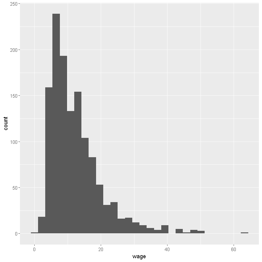
summary(df$wage)

ggplot(df, aes(x = wage))+ 
        geom_histogram(bins = 30)

shapiro.test(df$wage)

   Min. 1st Qu.  Median    Mean 3rd Qu.    Max. 
   0.84    6.92   10.08   12.37   15.63   64.08 

	Shapiro-Wilk normality test

data:  df$wage
W = 0.84488, p-value < 2.2e-16

library(moments)
skewness(df$wage)
kurtosis(df$wage)

1.848114127393

7.83656558034119

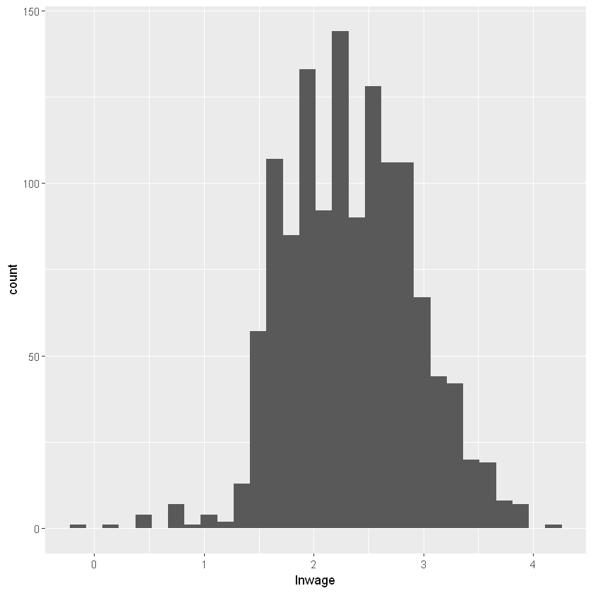
summary(df$lnwage)
skewness(df$lnwage)
kurtosis(df$lnwage)

ggplot(df, aes(x = lnwage))+ 
        geom_histogram(bins = 30)

   Min. 1st Qu.  Median    Mean 3rd Qu.    Max. 
-0.1744  1.9344  2.3106  2.3424  2.7492  4.1601 

0.0133949929381925

3.22633731089373

library('tseries')
jarque.bera.test(df$lnwage)
shapiro.test(df$lnwage)

Registered S3 method overwritten by 'quantmod':
  method            from
  as.zoo.data.frame zoo 

	Jarque Bera Test

data:  df$lnwage
X-squared = 2.7899, df = 2, p-value = 0.2478

	Shapiro-Wilk normality test

data:  df$lnwage
W = 0.99175, p-value = 1.268e-06

model4 <-  lm(lnwage~ female + nonwhite + union + education + exper, data = df)
tidy(model4)
glance(model4)

A tibble: 6 × 5

term	estimate	std.error	statistic	p.value
<chr>	<dbl>	<dbl>	<dbl>	<dbl>
(Intercept)	0.90550368	0.074174901	12.207683	1.662727e-32
female	-0.24915404	0.026625019	-9.357891	3.511043e-20
nonwhite	-0.13353510	0.037181913	-3.591399	3.413335e-04
union	0.18020354	0.036954854	4.876316	1.216066e-06
education	0.09987030	0.004812460	20.752442	1.025031e-82
exper	0.01276009	0.001171825	10.889073	1.795174e-26

A tibble: 1 × 12

r.squared	adj.r.squared	sigma	statistic	p.value	df	logLik	AIC	BIC	deviance	df.residual	nobs
<dbl>	<dbl>	<dbl>	<dbl>	<dbl>	<dbl>	<dbl>	<dbl>	<dbl>	<dbl>	<int>	<int>
0.3456505	0.3431004	0.4752374	135.5452	1.738922e-115	5	-867.0651	1748.13	1784.261	289.7663	1283	1289

education coefficient of 0.0999 suggests that for every additional year of schooling, the average wage rate goes up by about 9.99%, ceteris paribus

female dummy coefficient of –0.2492 as suggesting that the average female wage rate is lower by 24.92% as compared to the male average wage rate. (approximately)

(exp(-0.2492) - 1) * 100

-22.0575927019416

average female wage rate is lower by 22% as compared to the male average wage rate. (exact)

Dummy variables in structural change

\[ GPI_t = B_1 + B_2GPS_t +u_t, \]

GPS: gross private savings
GPI: gross private investments

df2 <- read_excel("data/Table3_6.xls")
head(df2,3)

A tibble: 3 × 5

obs	gpi	gps	recession81	gpsrec81
<dbl>	<dbl>	<dbl>	<dbl>	<dbl>
1959	78.5	84.6	0	0
1960	78.9	84.8	0	0
1961	78.2	91.8	0	0

model5 <- lm(gpi ~ gps, data = df2)
tidy(model5)
glance(model5)

A tibble: 2 × 5

term	estimate	std.error	statistic	p.value
<chr>	<dbl>	<dbl>	<dbl>	<dbl>
(Intercept)	-78.721047	27.48474252	-2.864173	6.230637e-03
gps	1.107395	0.02907993	38.081092	5.567391e-37

A tibble: 1 × 12

r.squared	adj.r.squared	sigma	statistic	p.value	df	logLik	AIC	BIC	deviance	df.residual	nobs
<dbl>	<dbl>	<dbl>	<dbl>	<dbl>	<dbl>	<dbl>	<dbl>	<dbl>	<dbl>	<int>	<int>
0.9686074	0.9679395	114.8681	1450.17	5.567391e-37	1	-300.9524	607.9049	613.5803	620149.8	47	49

if GPS increases by a dollar, the average GPI goes up by about $1.10.

Check for structural break

\[ GPI_t = B_1 + B_2GPS_t + \beta_3 \text{Recession81}_t + u_t, \]

GPS: gross private savings
GPI: gross private investments
Recession81: 0 before year 1981, 1 afterwords

model6 <- lm(gpi ~ gps + recession81, data = df2)
tidy(model6)
glance(model6)

A tibble: 3 × 5

term	estimate	std.error	statistic	p.value
<chr>	<dbl>	<dbl>	<dbl>	<dbl>
(Intercept)	-83.486025	23.15912656	-3.604887	7.649795e-04
gps	1.288672	0.04706553	27.380380	4.045379e-30
recession81	-240.787848	53.39662813	-4.509420	4.464419e-05

A tibble: 1 × 12

r.squared	adj.r.squared	sigma	statistic	p.value	df	logLik	AIC	BIC	deviance	df.residual	nobs
<dbl>	<dbl>	<dbl>	<dbl>	<dbl>	<dbl>	<dbl>	<dbl>	<dbl>	<dbl>	<int>	<int>
0.9782308	0.9772843	96.68906	1033.538	5.893647e-39	2	-291.9836	591.9672	599.5345	430043.7	46	49

Intercept pre recession: -83
Intercept post recession: (-83-240) = -324

To check for slope:

\[ GPI_t = B_1 + B_2GPS_t + \beta_3 \text{Recession81}_t + \beta_4 \text{GPS * Recession81}+ u_t, \]

model7 <- lm(gpi ~ gps + recession81 + gps*recession81, data = df2)
tidy(model7)
glance(model7)

A tibble: 4 × 5

term	estimate	std.error	statistic	p.value
<chr>	<dbl>	<dbl>	<dbl>	<dbl>
(Intercept)	-7.7798689	38.4495931	-0.2023394	8.405634e-01
gps	0.9510818	0.1474505	6.4501785	6.686678e-08
recession81	-357.4586528	70.2863017	-5.0857513	6.910536e-06
gps:recession81	0.3719201	0.1547662	2.4031102	2.044029e-02

A tibble: 1 × 12

r.squared	adj.r.squared	sigma	statistic	p.value	df	logLik	AIC	BIC	deviance	df.residual	nobs
<dbl>	<dbl>	<dbl>	<dbl>	<dbl>	<dbl>	<dbl>	<dbl>	<dbl>	<dbl>	<int>	<int>
0.9807067	0.9794205	92.03045	762.4731	1.42319e-38	3	-289.0255	588.051	597.5101	381132.2	45	49

GPI pre recession: -7.78 + 0.95 GPS
GPI post recession: (-7.78 - 357.45) + (0.95 + 0.37) GPS

Dummy variables in seasonal data (deseasonalization)

df3 <- read_excel("data/Table3_10.xls")
head(df3,3)

A tibble: 3 × 10

obs	sales	rpdi	conf	d2	d3	d4	lnsales	yearq	trend
<chr>	<dbl>	<dbl>	<dbl>	<dbl>	<dbl>	<dbl>	<dbl>	<dbl>	<dbl>
1986:1	53.714	84.18	286.6	0	0	0	3.983674	21916	1
1986:2	71.501	85.04	290.3	1	0	0	4.269711	21916	2
1986:3	96.374	84.57	284.5	0	1	0	4.568236	21916	3

\[ Sales_t = A_1 + A_2D_{2t} + A_3D_{3t} + A_4D_{4t} + u_t \]

\(D_2\) = 1 for second quarter
\(D_3\) = 1 for third quarter
\(D_4\) = 1 for fourth quarter

model8 <- lm(sales ~  d2 + d3 + d4, data = df3)
tidy(model8)
glance(model8)

A tibble: 4 × 5

term	estimate	std.error	statistic	p.value
<chr>	<dbl>	<dbl>	<dbl>	<dbl>
(Intercept)	73.18343	3.977483	18.399433	1.178376e-15
d2	14.69229	5.625010	2.611957	1.528526e-02
d3	27.96472	5.625010	4.971496	4.468310e-05
d4	57.11472	5.625010	10.153709	3.646049e-10

A tibble: 1 × 12

r.squared	adj.r.squared	sigma	statistic	p.value	df	logLik	AIC	BIC	deviance	df.residual	nobs
<dbl>	<dbl>	<dbl>	<dbl>	<dbl>	<dbl>	<dbl>	<dbl>	<dbl>	<dbl>	<int>	<int>
0.8234883	0.8014244	10.52343	37.32278	3.372103e-09	3	-103.4731	216.9462	223.6072	2657.822	24	28

Interpretation ofD2 is that the mean sales value in the second quarter is greater than the mean sales in the first, or reference, quarter by 14.69229 units; the actual mean sales value in the second quarter is (73.18343 + 14.69229) = 87.87572.

Deseasonalize

1. obtain estimated sales volume

2. obtain residuals (actual sales - estimated sales)

3. add mean value of sales to residuals

augmented <- augment(model8)

augmented <- augmented %>%
mutate(deseasonalized_sales = .resid + mean(augmented$sales))

head(augmented)

A tibble: 6 × 11

sales	d2	d3	d4	.fitted	.resid	.hat	.sigma	.cooksd	.std.resid	deseasonalized_sales
<dbl>	<dbl>	<dbl>	<dbl>	<dbl>	<dbl>	<dbl>	<dbl>	<dbl>	<dbl>	<dbl>
53.714	0	0	0	73.18343	-19.469427	0.1428571	9.814778	0.166390008	-1.9983394	78.65693
71.501	1	0	0	87.87571	-16.374714	0.1428571	10.097357	0.117697809	-1.6806985	81.75164
96.374	0	1	0	101.14814	-4.774144	0.1428571	10.695856	0.010004880	-0.4900175	93.35221
125.041	0	0	1	130.29814	-5.257143	0.1428571	10.684361	0.012131669	-0.5395925	92.86921
78.610	0	0	0	73.18343	5.426573	0.1428571	10.680063	0.012926240	0.5569827	103.55293
89.609	1	0	0	87.87571	1.733287	0.1428571	10.742676	0.001318749	0.1779044	99.85964

Expanded sales function

Frisch_Waugh Theorem

model9 <- lm(sales ~  rpdi + conf+ d2 + d3 + d4, data = df3)
tidy(model9)
glance(model9)

A tibble: 6 × 5

term	estimate	std.error	statistic	p.value
<chr>	<dbl>	<dbl>	<dbl>	<dbl>
(Intercept)	-152.9292193	52.59149307	-2.907870	8.156667e-03
rpdi	1.5989033	0.37015528	4.319547	2.764247e-04
conf	0.2939096	0.08437568	3.483344	2.106581e-03
d2	15.0452205	4.31537708	3.486421	2.091102e-03
d3	26.0024741	4.32524385	6.011794	4.741138e-06
d4	60.8722628	4.42743714	13.748871	2.795431e-12

A tibble: 1 × 12

r.squared	adj.r.squared	sigma	statistic	p.value	df	logLik	AIC	BIC	deviance	df.residual	nobs
<dbl>	<dbl>	<dbl>	<dbl>	<dbl>	<dbl>	<dbl>	<dbl>	<dbl>	<dbl>	<int>	<int>
0.9053748	0.883869	8.047637	42.09922	1.53222e-10	5	-94.74461	203.4892	212.8146	1424.818	22	28

Piecewise Linear Regression

introduce threshold (knot)

df4 <- read_excel("data/Table3_16.xls")
head(df4)

A tibble: 6 × 6

obs	avgcost	lotsize	z	d	zd
<dbl>	<dbl>	<dbl>	<dbl>	<dbl>	<dbl>
1	9.73	100	-100	0	0
2	9.61	120	-80	0	0
3	8.15	140	-60	0	0
4	6.98	160	-40	0	0
5	5.87	180	-20	0	0
6	4.98	200	0	0	0

ggplot(df4, aes(x = lotsize, y = avgcost)) +
geom_point()

\[ Y_i = \beta_0 + \beta_1 X_i + \beta_2(X_i-X^*)D_i + u_i \]

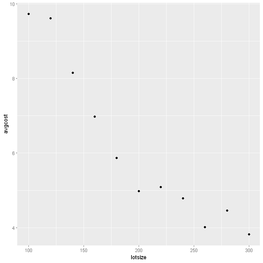
Y = average production cost,
X = lot size,
X* = threshold value of lot size,
D = 1 if Xi > X*
D = 0 if Xi < X

model10 <- lm(avgcost ~ lotsize, data = df4)
tidy(model10)
glance(model10)

A tibble: 2 × 5

term	estimate	std.error	statistic	p.value
<chr>	<dbl>	<dbl>	<dbl>	<dbl>
(Intercept)	12.29090855	0.749146219	16.406555	5.167361e-08
lotsize	-0.03077273	0.003571414	-8.616397	1.217549e-05

A tibble: 1 × 12

r.squared	adj.r.squared	sigma	statistic	p.value	df	logLik	AIC	BIC	deviance	df.residual	nobs
<dbl>	<dbl>	<dbl>	<dbl>	<dbl>	<dbl>	<dbl>	<dbl>	<dbl>	<dbl>	<int>	<int>
0.8918819	0.8798688	0.7491462	74.2423	1.217549e-05	1	-11.3276	28.65521	29.84889	5.050981	9	11

model10 <- lm(avgcost ~ lotsize + zd, data = df4)
tidy(model10)
glance(model10)

A tibble: 3 × 5

term	estimate	std.error	statistic	p.value
<chr>	<dbl>	<dbl>	<dbl>	<dbl>
(Intercept)	15.11647994	0.535382569	28.234912	2.674940e-09
lotsize	-0.05019853	0.003332127	-15.065011	3.726359e-07
zd	0.03885161	0.005945966	6.534112	1.814740e-04

A tibble: 1 × 12

r.squared	adj.r.squared	sigma	statistic	p.value	df	logLik	AIC	BIC	deviance	df.residual	nobs
<dbl>	<dbl>	<dbl>	<dbl>	<dbl>	<dbl>	<dbl>	<dbl>	<dbl>	<dbl>	<int>	<int>
0.9829381	0.9786727	0.3156508	230.4409	8.474347e-08	2	-1.172523	10.34505	11.93663	0.7970835	8	11

lot size < 200
Average cost = 15.1164 – 0.0502 lot size,

lot size > 200
Average cost = (15.1164 – 0.0385 × 200) + (–0.0502 + 0.0388) lot size = 7.4164 – 0.0114 lot size,

up to a lot size of 200 units, the unit cost decreases by 5 cents per unit increase in the lot size, but beyond the lot size of 200 units, it decreases only by about 1 cent

Exercises

🚧 Under Construction