4. multicollinearity

suppressPackageStartupMessages({
  library(tidyverse)
  library(tidymodels)
  library(readxl)
  library(multcomp)
  library(car)
})

df <- read_excel("data/Table4_2.xls")
head(df,3)

A tibble: 3 × 3

expend	income	wealth
<dbl>	<dbl>	<dbl>
70	80	810
65	100	1009
90	120	1273

model <- lm(expend ~ income + wealth, data = df)
tidy(model)
glance(model)$r.squared

A tibble: 3 × 5

term	estimate	std.error	statistic	p.value
<chr>	<dbl>	<dbl>	<dbl>	<dbl>
(Intercept)	24.77473327	6.75249960	3.6689722	0.007975077
income	0.94153734	0.82289826	1.1441722	0.290164748
wealth	-0.04243453	0.08066448	-0.5260621	0.615094539

0.963504395243514

none of the slope coeffi cients is statistically signifi cant, as the t values are statistically insignificant. Yet the R2 value is very high.

model2 <- lm(expend ~ income, data = df)
tidy(model2)
glance(model2)$r.squared

A tibble: 2 × 5

term	estimate	std.error	statistic	p.value
<chr>	<dbl>	<dbl>	<dbl>	<dbl>
(Intercept)	24.4545455	6.41381730	3.812791	5.142172e-03
income	0.5090909	0.03574281	14.243171	5.752746e-07

0.962061560486757

income alone has significant impact on expenditure,

model3 <- lm(expend ~ wealth, data = df)
tidy(model3)
glance(model3)$r.squared

A tibble: 2 × 5

term	estimate	std.error	statistic	p.value
<chr>	<dbl>	<dbl>	<dbl>	<dbl>
(Intercept)	24.41104485	6.874096840	3.551164	7.496699e-03
wealth	0.04976377	0.003743986	13.291656	9.802080e-07

0.956679038871206

wealth alone has a significant impact on expenditure

model4 <- lm(wealth ~ income, data = df)
tidy(model4)
glance(model4)$r.squared

A tibble: 2 × 5

term	estimate	std.error	statistic	p.value
<chr>	<dbl>	<dbl>	<dbl>	<dbl>
(Intercept)	7.545455	29.4758107	0.255988	8.044195e-01
income	10.190909	0.1642623	62.040474	5.064901e-12

0.997925860058925

wealth and income are highly related

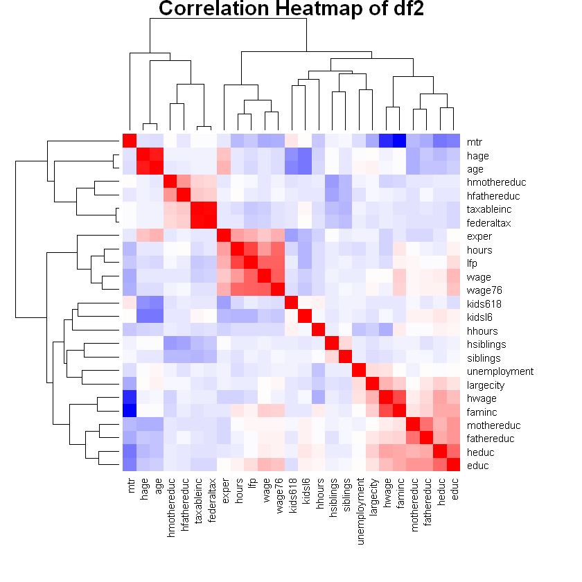
Example

df2 <- read_excel("data/Table4_4.xls")
head(df2,3)

A tibble: 3 × 25

taxableinc	federaltax	hsiblings	hfathereduc	hmothereduc	siblings	lfp	hours	kidsl6	kids618	⋯	hage	heduc	hwage	faminc	mtr	mothereduc	fathereduc	unemployment	largecity	exper
<dbl>	<dbl>	<dbl>	<dbl>	<dbl>	<dbl>	<dbl>	<dbl>	<dbl>	<dbl>	⋯	<dbl>	<dbl>	<dbl>	<dbl>	<dbl>	<dbl>	<dbl>	<dbl>	<dbl>	<dbl>
12200	1494	1	14	16	4	1	1610	1	0	⋯	34	12	4.0288	16310	0.7215	12	7	5	0	14
18000	2615	8	7	3	0	1	1656	0	2	⋯	30	9	8.4416	21800	0.6615	7	7	11	1	5
24000	3957	4	7	10	2	1	1980	1	3	⋯	40	12	3.5807	21040	0.6915	12	7	5	0	15

Hours: hours worked in 1975 (dependent variable)
Kidslt6: number of kids under age 6
Kidsge6: number of kids between ages 6 and 18
Age: woman’s age in years
Educ: years of schooling
Wage: estimated wage from earnings
Hushrs: hours worked by husband
Husage: husband’s age
Huseduc: husband’s years of schooling
Huswage: husband’s hourly wage, 1975
Faminc: family income in 1975
Mtr: federal marginal tax rate facing a woman
motheduc: mother’s years of schooling
fatheduc: father’s years of schooling
Unem: unemployment rate in county of residence
exper: actual labor market experience

assess the impact of several socio-economic variables on married women’s hours of work in the labor market. This is cross-sectional data on 753 married women for the year 1975. It should be noted that there were 325 married women who did not work and hence had zero hours of work.

model5 <- lm(hours ~ age + educ + exper + faminc + fathereduc + 
            hage + heduc + hhours + hwage + kidsl6 + kids618 +
            wage + mothereduc + mtr + unemployment, data = df2)

tidy(model5)
glance(model5)

A tibble: 16 × 5

term	estimate	std.error	statistic	p.value
<chr>	<dbl>	<dbl>	<dbl>	<dbl>
(Intercept)	5805.4723070	6.843439e+02	8.4832671	1.194368e-16
age	-24.0044110	6.859174e+00	-3.4996069	4.939481e-04
educ	-13.7760578	1.528931e+01	-0.9010257	3.678690e-01
exper	34.9538799	3.456319e+00	10.1130377	1.331411e-22
faminc	0.0156683	4.641855e-03	3.3754394	7.755884e-04
fathereduc	-4.8206771	8.673176e+00	-0.5558145	5.785063e-01
hage	-5.0282298	6.669922e+00	-0.7538664	4.511702e-01
heduc	-11.6952485	1.101195e+01	-1.0620504	2.885607e-01
hhours	-0.3389067	5.107115e-02	-6.6359714	6.246245e-11
hwage	-107.3373543	1.091622e+01	-9.8328291	1.600070e-21
kidsl6	-322.7168869	5.345385e+01	-6.0372993	2.482936e-09
kids618	-4.0422005	2.149471e+01	-0.1880556	8.508849e-01
wage	51.6767604	8.714492e+00	5.9299799	4.655600e-09
mothereduc	9.8422151	9.195859e+00	1.0702878	2.848402e-01
mtr	-3956.7686273	7.215385e+02	-5.4837941	5.723755e-08
unemployment	-7.6865804	7.979074e+00	-0.9633424	3.356917e-01

A tibble: 1 × 12

r.squared	adj.r.squared	sigma	statistic	p.value	df	logLik	AIC	BIC	deviance	df.residual	nobs
<dbl>	<dbl>	<dbl>	<dbl>	<dbl>	<dbl>	<dbl>	<dbl>	<dbl>	<dbl>	<int>	<int>
0.434307	0.4227936	661.9732	37.72179	8.317512e-81	15	-5951.279	11936.56	12015.17	322959634	737	753

colnames(df2)

1. 'taxableinc'
2. 'federaltax'
3. 'hsiblings'
4. 'hfathereduc'
5. 'hmothereduc'
6. 'siblings'
7. 'lfp'
8. 'hours'
9. 'kidsl6'
10. 'kids618'
11. 'age'
12. 'educ'
13. 'wage'
14. 'wage76'
15. 'hhours'
16. 'hage'
17. 'heduc'
18. 'hwage'
19. 'faminc'
20. 'mtr'
21. 'mothereduc'
22. 'fathereduc'
23. 'unemployment'
24. 'largecity'
25. 'exper'

df2 %>%
  summarize(correlation = cor(hage, faminc, use = "complete.obs"))

A tibble: 1 × 1

correlation
<dbl>
0.04050263

correlation_matrix <- cor(df2, use = "complete.obs")

heatmap(correlation_matrix, 
        col = colorRampPalette(c("blue", "white", "red"))(100),
        symm = TRUE,         
        margins = c(8, 8),   
        main = "Correlation Heatmap of df2")

vif(model5)

age

5.26144147726373

educ

2.0858157402719

exper

1.33480562987452

faminc

5.49467416520725

fathereduc

1.64735313494315

hage

4.95813811611547

heduc

1.89893838127637

hhours

1.58762941970657

hwage

3.65996838421493

kidsl6

1.34613841992449

kids618

1.3812278886656

wage

1.36962420005194

mothereduc

1.6456166790573

mtr

6.22848954766369

unemployment

1.06008242126237

model6 <- lm(hours ~ age + educ + exper + faminc + hhours + hwage + kidsl6  +
            wage  + mtr + unemployment, data = df2)

tidy(model6)
glance(model6)

A tibble: 11 × 5

term	estimate	std.error	statistic	p.value
<chr>	<dbl>	<dbl>	<dbl>	<dbl>
(Intercept)	5.720767e+03	6.622272e+02	8.6386770	3.464404e-17
age	-2.823358e+01	3.566101e+00	-7.9172148	8.858432e-15
educ	-1.828395e+01	1.223935e+01	-1.4938658	1.356358e-01
exper	3.511494e+01	3.394298e+00	10.3452722	1.595033e-23
faminc	1.592231e-02	4.509078e-03	3.5311679	4.392850e-04
hhours	-3.461675e-01	5.018601e-02	-6.8976900	1.132866e-11
hwage	-1.100438e+02	1.066498e+01	-10.3182403	2.040707e-23
kidsl6	-3.193502e+02	5.231116e+01	-6.1048203	1.658396e-09
wage	5.188557e+01	8.657064e+00	5.9934370	3.204685e-09
mtr	-3.929831e+03	6.850461e+02	-5.7365936	1.406737e-08
unemployment	-7.721889e+00	7.940710e+00	-0.9724432	3.311470e-01

A tibble: 1 × 12

r.squared	adj.r.squared	sigma	statistic	p.value	df	logLik	AIC	BIC	deviance	df.residual	nobs
<dbl>	<dbl>	<dbl>	<dbl>	<dbl>	<dbl>	<dbl>	<dbl>	<dbl>	<dbl>	<int>	<int>
0.432122	0.4244687	661.0119	56.46187	1.932607e-84	10	-5952.73	11929.46	11984.95	324207062	742	753

vif(model6)

age

1.42629876639497

educ

1.34053961380487

exper

1.29107879991459

faminc

5.19991905936222

hhours

1.53753610679107

hwage

3.50360087467717

kidsl6

1.29295288892452

wage

1.35556617939112

mtr

5.63073994873757

unemployment

1.05296872093097

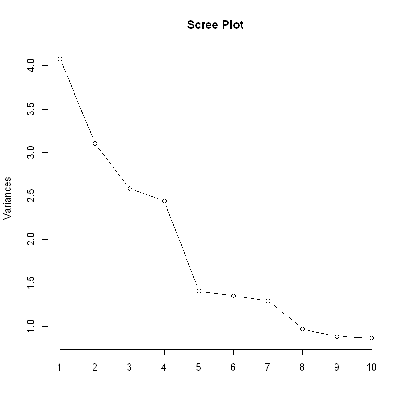
Principal components analysis

Results are different from the book

scaled_data <- scale(df2)

pca_result <- prcomp(scaled_data, center = TRUE, scale = TRUE)

pca_components <- pca_result$rotation

# Extract standardized scores (principal component scores)
pca_scores <- pca_result$x

# Extract standard deviations of principal components
pca_std_dev <- pca_result$sdev

variance_explained <- pca_std_dev^2 / sum(pca_std_dev^2)

screeplot(pca_result, type = "lines", main = "Scree Plot")

summary(pca_result)

Importance of components:
                         PC1    PC2    PC3     PC4     PC5     PC6     PC7
Standard deviation     2.019 1.7615 1.6080 1.56381 1.18734 1.16346 1.13759
Proportion of Variance 0.163 0.1241 0.1034 0.09782 0.05639 0.05415 0.05176
Cumulative Proportion  0.163 0.2871 0.3906 0.48837 0.54476 0.59891 0.65067
                           PC8     PC9    PC10    PC11    PC12    PC13    PC14
Standard deviation     0.98662 0.93992 0.93027 0.88700 0.85488 0.83909 0.79942
Proportion of Variance 0.03894 0.03534 0.03462 0.03147 0.02923 0.02816 0.02556
Cumulative Proportion  0.68961 0.72495 0.75956 0.79103 0.82027 0.84843 0.87399
                          PC15    PC16    PC17   PC18    PC19    PC20    PC21
Standard deviation     0.77286 0.71328 0.65361 0.6285 0.58349 0.56742 0.44504
Proportion of Variance 0.02389 0.02035 0.01709 0.0158 0.01362 0.01288 0.00792
Cumulative Proportion  0.89788 0.91824 0.93532 0.9511 0.96474 0.97762 0.98554
                          PC22    PC23    PC24    PC25
Standard deviation     0.35882 0.32453 0.31267 0.17204
Proportion of Variance 0.00515 0.00421 0.00391 0.00118
Cumulative Proportion  0.99069 0.99491 0.99882 1.00000

Exercises

🚧 Under Construction